Valvulopathies

Created March 2024

The goal of this tutorial is to learn how to simulate valvular pathologies using the CircAdapt framework. This tutorial assumes basic knowledge on Python and the VanOsta2024 model as provided in the previous tutorial named ‘Basics to Python and CircAdapt’.

This tutorial assumes the installation is followed as described on the CircAdapt framework webstite (https://framework.circadapt.org/latest/userguide/installation.html). This uses Python >3.9 installed with anaconda and editted in Spyder. Other ways are possible, but might not be in line with this tutorial.

Content

1. Healthy reference

2. Aortic stenosis

3. Mitral regurgitation

First, we import all needed modules according to convention at the start of the script. We will define the VanOsta2024 model and run this model.

import circadapt
import matplotlib.pyplot as plt
import numpy as np

from circadapt import VanOsta2024
model = VanOsta2024()

model.run(stable = True)

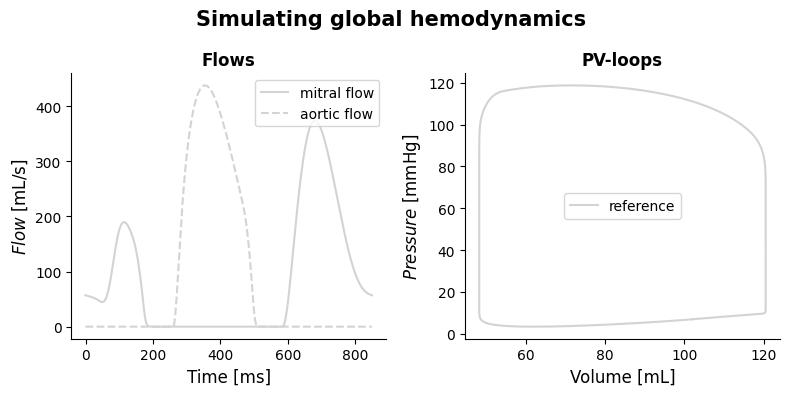
Plot healthy reference hemodynamics

Now we obtain our hemodynamic signals and plot them for the healthy reference simulation.

# get all pressure signals 
pressures = model['Cavity']['p'][:, ['cLv', 'La', 'SyArt']]*7.5e-3
p_lv, p_la, p_ao = pressures.T

# get LV volume
V_lv = model['Cavity']['V'][:, 'cLv']*1e6

# get transvalvular flow 
flows = model['Valve']['q'][:, ['LaLv', 'LvSyArt']]*1e6
q_mv, q_ao = flows.T

# get time
time = model['Solver']['t']*1e3

# Plot hemodynamics 

fig = plt.figure(1, figsize=(8, 4))
ax1 = fig.add_subplot(1, 2, 1)
ax2 = fig.add_subplot(1, 2, 2)

# Plot transvalvular flows
ax1.plot(time, q_mv, color = 'lightgrey', linestyle = '-', label = 'mitral flow')
ax1.plot(time, q_ao, color = 'lightgrey', linestyle = '--', label = 'aortic flow')
ax1.legend()

# Plot PV loops
ax2.plot(V_lv, p_lv, color = 'lightgrey', label = 'reference')
ax2.legend()

# plot design, add labels
for ax in [ax1, ax2]:
    ax.spines[['right', 'top']].set_visible(False)
ax1.set_xlabel('Time [ms]', fontsize=12)
ax2.set_xlabel('Volume [mL]', fontsize=12)

ax1.set_ylabel('$Flow$ [mL/s]', fontsize=12)
ax2.set_ylabel('$Pressure$ [mmHg]', fontsize=12)

ax1.set_title('Flows',
             fontsize=12, fontweight='bold')
ax2.set_title('PV-loops',
             fontsize=12, fontweight='bold')

fig.suptitle('Simulating global hemodynamics ',
             fontsize=15, fontweight='bold')

plt.tight_layout()
plt.draw()

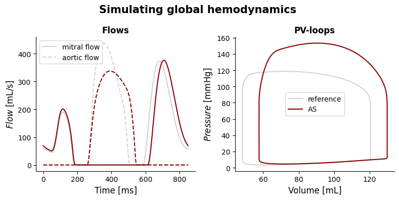
Simulating aortic stenosis

In case of an aortic stenosis, the effective orifice area (EOA) of the aortic valve is reduced. In this tutorial, we assume a reduction in EOA of 80%.

First, we have to change EOA for the aortic valve and then run the model until it is hemodynamically stable.

# get reference value for aortic EOA
model = VanOsta2024() # to make sure the right reference value is taken 
model.run(stable = True)

EOA_ao_ref = model['Valve']['A_open']['LvSyArt']

# reduce aortic EOA by 80% and assign as new EOA
model['Valve']['A_open']['LvSyArt'] = 0.2*EOA_ao_ref

model.run(stable = True)

After the model has run, we again obtain the newly simulated hemodynamic signals and plot them in the figure above.

# get all pressure signals 
pressures = model['Cavity']['p'][:, ['cLv', 'La', 'SyArt']]*7.5e-3
p_lv, p_la, p_ao = pressures.T

# get LV volume
V_lv = model['Cavity']['V'][:, 'cLv']*1e6

# get transvalvular flow 
flows = model['Valve']['q'][:, ['LaLv', 'LvSyArt']]*1e6
q_mv, q_ao = flows.T

# get time
time = model['Solver']['t']*1e3

# Plot hemodynamics 

# Plot transvalvular flows
ax1.plot(time, q_mv, color = 'darkred', linestyle = '-', label = 'mitral flow')
ax1.plot(time, q_ao, color = 'darkred', linestyle = '--', label = 'aortic flow')

# Plot PV loops
ax2.plot(V_lv, p_lv, color = 'darkred', label = 'AS')
ax2.legend()

fig

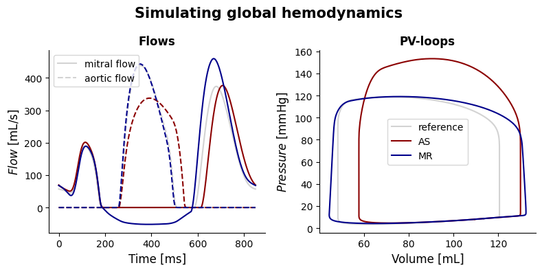
Simulating mitral regurgitation (MR)

In case of a mitral regurgitation, the effective regurgitant orifice area (EROA) of the mitral valve is increased. In this tutorial, we assume an EROA of 0.1 cm2.

First, we have to change EROA for the mitral valve and then run the model until it is hemodynamically stable.

# get reference value for mitral EROA
model = VanOsta2024() # to make sure the right reference value is taken 
model.run(stable = True)

# set mitral EROA to 0.1 cm2 and assign as new EROA
model['Valve']['A_leak']['LaLv'] = 0.1e-4
model.run(stable = True)

After the model has run, we again obtain the newly simulated hemodynamic signals and plot them in the figure above.

# get all pressure signals 
pressures = model['Cavity']['p'][:, ['cLv', 'La', 'SyArt']]*7.5e-3
p_lv, p_la, p_ao = pressures.T

# get LV volume
V_lv = model['Cavity']['V'][:, 'cLv']*1e6

# get transvalvular flow 
flows = model['Valve']['q'][:, ['LaLv', 'LvSyArt']]*1e6
q_mv, q_ao = flows.T

# get time
time = model['Solver']['t']*1e3

# Plot hemodynamics 

# Plot transvalvular flows
ax1.plot(time, q_mv, color = 'darkblue', linestyle = '-', label = 'mitral flow')
ax1.plot(time, q_ao, color = 'darkblue', linestyle = '--', label = 'aortic flow')

# Plot PV loops
ax2.plot(V_lv, p_lv, color = 'darkblue', label = 'MR')
ax2.legend()

fig