Timings module

The Timings module controls the contraction of a physiological heart beat. It assumes homogeneous contraction within a Wall segment, even when more Patch objects are simulated within a single Wall segment. The Timings module does control the atrial-ventricular delay and heartrate-dependent parameters.

Lets create the model.

import circadapt
import matplotlib.pyplot as plt
import numpy as np

model = circadapt.VanOsta2024()

Model implementation

When using the Timings module, each connected Wall will be triggered once during the cycle. By this defenition, the cycle time of the model t_cycle is equal to 60 / t_cycle. We will simulate a heart rate of 75 bpm. In this tutorial, we will turn pressure-flow regulation off.

         model['General']['t_cycle'] = 60 / 75
         model['PFC']['is_active'] = False

AV-delay

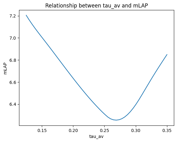
The atrio-ventricular (AV) delay is controlled by the Timings module. By default, when law_tau_av==1, the AV-delay is set to tau_av = c_tau_av1 * t_cycle + c_tau_av0 + dtau_av. Alternatively, when law_tau_av==2, the AV-delay is set to tau_av = c_tau_av1 / t_cycle + c_tau_av0 + dtau_av. When law_tau_av==0, the AV-delay is not controlled meaning tau_av is a input parameter. To investigate the effect of different AV-delays on mean left atrial pressure, you can turn off the AV-delay control.

model['Timings']['law_tau_av'] = 0

tau_avs = np.linspace(0.125, 0.35, 51)
mLAP = np.empty_like(tau_avs)

for i, tau_av in enumerate(tau_avs):
    model['Timings']['tau_av'] = tau_av

    model.run(stable=True)

    mLAP[i] = np.mean(model['Cavity']['p'][:, 'La']) / 133

Now, we can plot this relationship:

plt.plot(tau_avs, mLAP)
plt.xlabel("tau_av")
plt.ylabel("mLAP")
plt.title("Relationship between tau_av and mLAP")

Text(0.5, 1.0, 'Relationship between tau_av and mLAP')

Different AV-delay relationships

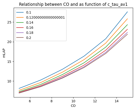
In studies with varying t_cycle, changing the AV-delay relationship can be of interest. In this example, we will plot the mLAP - CO relationship for various AV-delay relationships.

c_tau_av1s = np.linspace(0.1, 0.2, 6)
COs = np.linspace(5, 15, 6)

mLAP = np.empty((*c_tau_av1s.shape, *COs.shape))

for i, c_tau_av1 in enumerate(c_tau_av1s):
    for j, CO in enumerate(COs):
        model = circadapt.VanOsta2024()
        model['Timings']['law_tau_av'] = 1
        model['Timings']['c_tau_av1'] = c_tau_av1
        model['PFC']['is_active'] = True
        model['PFC']['q0'] = CO / 60e3
        model['General']['t_cycle'] = 1/3 * 0.85 + 2/3 * 0.85 / (CO / 5)
        try:
            model.run(stable=True)
            mLAP[i, j] = np.mean(model['Cavity']['p'][:, 'La']) / 133
        except circadapt.error.ModelCrashed:
            mLAP[i, j] = np.nan

 plt.plot(COs, mLAP.T, label=c_tau_av1s)
 plt.legend()
 plt.xlabel("CO")
 plt.ylabel("mLAP")
 plt.title("Relationship between CO and as function of c_tau_av1")

Text(0.5, 1.0, 'Relationship between CO and as function of c_tau_av1')

Relative contraction duration

Besides moment of contraction, also duration of contraction is scaled using the Timings module. The Timings module controls the time_act parameter of the Patch module. With law_ta == 0 and law_tv == 0, no t_cycle dependency is simulated. By default, law_ta = 1 and law_tv = 1, simulating the relative contraction duration by ta = (c_ta_rest * t_cycle_rest + c_ta_tcycle * t_cycle) * time_fac and tv = (c_tv_rest * t_cycle_rest + c_tv_tcycle * t_cycle) * time_fac.