Regional myocardial (dys)function
Created March 2024
The goal of this tutorial is to learn how to subdivide the cardiac walls into segments (so-called patches) that will allow you to simulate regional myocardial dysfunction using the CircAdapt framework. This tutorial assumes basic knowledge on Python and the VanOsta2024 model as provided in the previous tutorial named ‘Basics to Python and CircAdapt’.
This tutorial assumes the installation is followed as described on the CircAdapt framework webstite (https://framework.circadapt.org/latest/userguide/installation.html). This uses Python >3.9 installed with anaconda and editted in Spyder. Other ways are possible, but might not be in line with this tutorial.
Content
1. Healthy reference
2. Subdivide the cardiac walls into segments
3. Simulate and plot a left ventricular activation delay
First, we import all needed modules according to convention at the start of the script. We will define the VanOsta2024 model and run this model.
import circadapt
import matplotlib.pyplot as plt
import numpy as np

from circadapt import VanOsta2024
model = VanOsta2024()

model.run(stable = True)
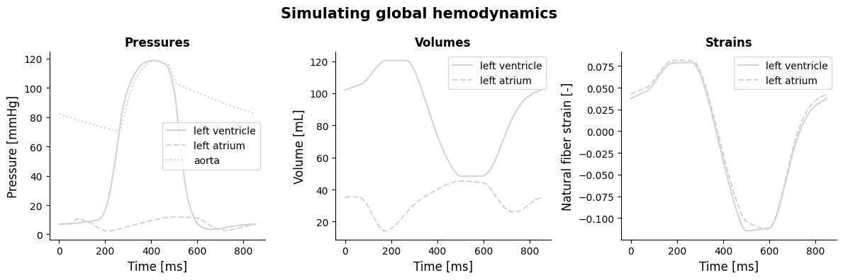
Plot healthy reference hemodynamics
Now we obtain our hemodynamic signals and plot them for the healthy reference simulation.
# get all pressure signals
pressures = model['Cavity']['p'][:, ['cLv', 'La', 'SyArt']]*7.5e-3
p_lv, p_la, p_ao = pressures.T

# get LV and LA volume
volumes = model['Cavity']['V'][:, ['cLv', 'La']]*1e6
V_lv, V_la = volumes.T

# get natural fiber strain
strains = model['Patch']['Ef'][:, ['pLv0', 'pSv0']]
Ef_lv, Ef_sv = strains.T

# get time
time = model['Solver']['t']*1e3
# Plot hemodynamics

fig = plt.figure(1, figsize=(12, 4))
ax1 = fig.add_subplot(1, 3, 1)
ax2 = fig.add_subplot(1, 3, 2)
ax3 = fig.add_subplot(1, 3, 3)

# Plot pressures
ax1.plot(time, p_lv, color = 'lightgrey', linestyle = '-', label = 'left ventricle')
ax1.plot(time, p_la, color = 'lightgrey', linestyle = '--', label = 'left atrium')
ax1.plot(time, p_ao, color = 'lightgrey', linestyle = ':', label = 'aorta')
ax1.legend()

# Plot volumes
ax2.plot(time, V_lv, color = 'lightgrey', linestyle = '-', label = 'left ventricle')
ax2.plot(time, V_la, color = 'lightgrey', linestyle = '--', label = 'left atrium')
ax2.legend()

# Plot strains
ax3.plot(time, Ef_lv, color = 'lightgrey', linestyle = '-', label = 'left ventricle')
ax3.plot(time, Ef_sv, color = 'lightgrey', linestyle = '--', label = 'left atrium')
ax3.legend()

# plot design, add labels
for ax in [ax1, ax2, ax3]:
    ax.spines[['right', 'top']].set_visible(False)
ax1.set_xlabel('Time [ms]', fontsize=12)
ax2.set_xlabel('Time [ms]', fontsize=12)
ax3.set_xlabel('Time [ms]', fontsize=12)

ax1.set_ylabel('Pressure [mmHg]', fontsize=12)
ax2.set_ylabel('Volume [mL]', fontsize=12)
ax3.set_ylabel('Natural fiber strain [-]', fontsize=12)

ax1.set_title('Pressures',
             fontsize=12, fontweight='bold')
ax2.set_title('Volumes',
             fontsize=12, fontweight='bold')
ax3.set_title('Strains',
             fontsize=12, fontweight='bold')

fig.suptitle('Simulating global hemodynamics ',
             fontsize=15, fontweight='bold')

plt.tight_layout()
plt.draw()
Subdivide the cardiac walls into segments
At baseline, the ventricular walls are subdivided into the right ventricle, left ventricle and intraventricular septum. In order to simulate differences within each of these walls, the wall should be subdivided into segments that can have their own properties. We take a left ventricular activation delay as an example in this tutorial. In this case, the intraventicular septum is first activated, after which the left ventricle is gradually activated as well. In order to simulate this, we divide the intraventricular septum in 6 segments and the left ventricle in 12 segments using the Patch component:
# divide the left ventricle (position 2) in 12 patches and the intraventricular septum (position 3) in 6 segments.
model = VanOsta2024()
model['Wall']['n_patch'][2:4] = [12, 6]

print('See how the LV and septal patches now have additional numbering: \n\n', model['Patch'].objects)

print('\nThe LV now corresponds to object numers 2:14 and the septum to objects 14:20.')
See how the LV and septal patches now have additional numbering:

 ['Model.Peri.La.wLa.pLa0', 'Model.Peri.Ra.wRa.pRa0', 'Model.Peri.TriSeg.wLv.pLv0', 'Model.Peri.TriSeg.wLv.pLv1', 'Model.Peri.TriSeg.wLv.pLv2', 'Model.Peri.TriSeg.wLv.pLv3', 'Model.Peri.TriSeg.wLv.pLv4', 'Model.Peri.TriSeg.wLv.pLv5', 'Model.Peri.TriSeg.wLv.pLv6', 'Model.Peri.TriSeg.wLv.pLv7', 'Model.Peri.TriSeg.wLv.pLv8', 'Model.Peri.TriSeg.wLv.pLv9', 'Model.Peri.TriSeg.wLv.pLv10', 'Model.Peri.TriSeg.wLv.pLv11', 'Model.Peri.TriSeg.wSv.pSv0', 'Model.Peri.TriSeg.wSv.pSv1', 'Model.Peri.TriSeg.wSv.pSv2', 'Model.Peri.TriSeg.wSv.pSv3', 'Model.Peri.TriSeg.wSv.pSv4', 'Model.Peri.TriSeg.wSv.pSv5', 'Model.Peri.TriSeg.wRv.pRv0']

The LV now corresponds to object numers 2:14 and the septum to objects 14:20.
Simulate a left ventricular activation delay
Now that we have subdivided the intraventricular septum and the left ventricle, we can assign different activation times to each patch. We can do this by changing ‘dt’ within the patch component.
Note that CircAdapt is a mechanical model, and does not incorporate electrical activation. Therefore, an activation delay refers to a delay in mechanical activation.
# let the septal activation time range between 0 and 0.01 sec
model['Patch']['dt'][14:20] = np.linspace(0, 0.01, 6)

# let the LV activation time range between 0.01 and 0.05 sec
model['Patch']['dt'][2:14]  = np.linspace(0.01, 0.05, 12)

print('See how the activation times change for each patch: \n', model['Patch']['dt'])
See how the activation times change for each patch:
 array([0.        , 0.        , 0.01      , 0.01363636, 0.01727273,
       0.02090909, 0.02454545, 0.02818182, 0.03181818, 0.03545455,
       0.03909091, 0.04272727, 0.04636364, 0.05      , 0.        ,
       0.002     , 0.004     , 0.006     , 0.008     , 0.01      ,
       0.        ])
# run the model and obtain hemodynamics

model.run(stable = True)

# get all pressure signals
pressures = model['Cavity']['p'][:, ['cLv', 'La', 'SyArt']]*7.5e-3
p_lv, p_la, p_ao = pressures.T

# get LV and LA volume
volumes = model['Cavity']['V'][:, ['cLv', 'La']]*1e6
V_lv, V_la = volumes.T

# get natural fiber strain
Ef_lv = model['Patch']['Ef'][:, 2:14]
Ef_sv = model['Patch']['Ef'][:, 14:20]

# get time
time = model['Solver']['t']*1e3
# and plot the results

# Plot transvalvular flows
ax1.plot(time, p_lv, color = 'darkred', linestyle = '-', label = 'left ventricle')
ax1.plot(time, p_la, color = 'darkred', linestyle = '--', label = 'left atrium')
ax1.plot(time, p_ao, color = 'darkred', linestyle = ':', label = 'aorta')


# Plot volumes
ax2.plot(time, V_lv, color = 'darkred', linestyle = '-', label = 'left ventricle')
ax2.plot(time, V_la, color = 'darkred', linestyle = '--', label = 'left atrium')


# Plot volumes
ax3.plot(time, Ef_lv, color = 'darkred', linestyle = '-', label = 'reference')
ax3.plot(time, Ef_sv, color = 'darkred', linestyle = '--', label = 'reference')

fig
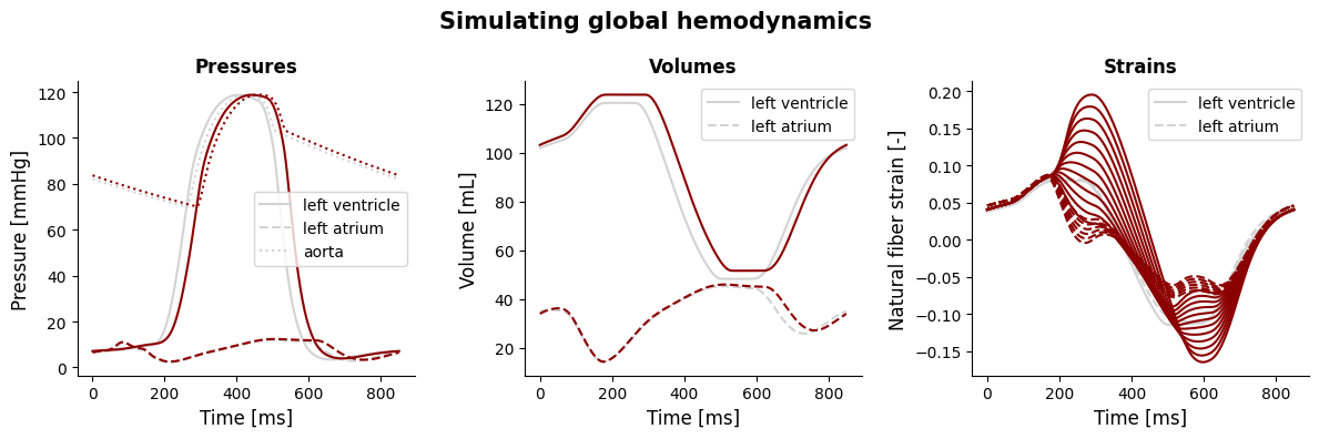
You can see that the strains show a very different behavior, attributable to the regional differences in activation time; the septal segments are activated earlier, causing shortening of the fibers (negative strain). Consequently, fibers in the LV free wall are stretched (positive strain). Then, the LV wall is activated as well, although later in time, causing a strong contraction as seen by the rapid decrease of left ventricular strains, thereby initially stretching the septal fibers.