Load experiment

Tags: PreAfterloadExperiment Patch2022

Tutorial on how to implement the preload-afterload experiment. This tutorial discusses how to build the model, how to switch between different patch types, and how to extract and plot information from the model.

Todo

Make Preload Afterload methods figure

As all projects, we start with importing packages.

1from circadapt import CircAdapt
2import numpy as np
3import matplotlib.pyplot as plt
4
5import time
6

We then create an empty model. Then, we add the PreAfterloadExperiment wall object. This object is empty by default, but it needs at least 1 patch object to work. In this tutorial, we use the Patch2022 object.

The model has to be parametized, as default parameter values do not make sense for this setup.

 1model.set('Model.t_cycle', 1e-0)
 2model.set('Solver.dt', 1e-3)
 3model.set('Solver.dt_export', 1e-3)
 4
 5model['LoadExperiment']['Am_ref_afterload'] =  0.006
 6model['LoadExperiment']['T_afterload'] =  200
 7model['LoadExperiment']['n_iter'] =  5
 8model['Patch']['Am_ref'] =  0.005
 9model['Patch']['V_wall'] = 92.43*1e-6
10model['Patch']['ADO'] = 3.0
11model['Patch']['tr'] = 0.5
12model['Patch']['td'] = 0.5
13model['Patch']['k1'] = 10.
14model['Patch']['v_max'] = 7.0
15model['Patch']['dt'] = 0.2
16
17model['Patch']['dt'] = [0.1, 0.1]
18
19model.set('Model.PAE.pAE0.l_si', -0.04 + 2 * np.sqrt(
20    model['LoadExperiment']['Am_ref_afterload'][0]/model['Patch']['Am_ref'][0]))
21model.set('Model.PAE.pAE1.l_si', model.get('Model.PAE.pAE0.l_si', dtype=float))
22
23

Now the model setup is finished and we can run the simulation. For this setup, only 1 run is sufficient.

1t0 = time.time()
2model.run(1)
3t1 = time.time()
4print(t1-t0)
5

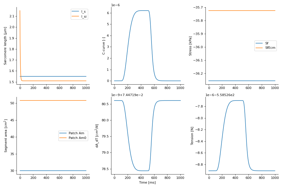
The simulation will result in the stresses and tensions shown in the plot below.

(Source code, png, hires.png, pdf)

../../../_images/Patch2022.png

The full code is shown below.

 1from circadapt import CircAdapt
 2import numpy as np
 3import matplotlib.pyplot as plt
 4
 5import time
 6
 7# %% Create custom model
 8model = CircAdapt('forward_euler')
 9model.add_component('LoadExperiment', 'PAE')
10model.add_component('Patch', 'P', 'PAE')
11
12model['LoadExperiment']['n_patch'] = 2
13
14
15# %% Set model parameters
16model.set('Model.t_cycle', 1e-0)
17model.set('Solver.dt', 1e-3)
18model.set('Solver.dt_export', 1e-3)
19
20model['LoadExperiment']['Am_ref_afterload'] =  0.006
21model['LoadExperiment']['T_afterload'] =  200
22model['LoadExperiment']['n_iter'] =  5
23model['Patch']['Am_ref'] =  0.005
24model['Patch']['V_wall'] = 92.43*1e-6
25model['Patch']['ADO'] = 3.0
26model['Patch']['tr'] = 0.5
27model['Patch']['td'] = 0.5
28model['Patch']['k1'] = 10.
29model['Patch']['v_max'] = 7.0
30model['Patch']['dt'] = 0.2
31
32model['Patch']['dt'] = [0.1, 0.1]
33
34model.set('Model.PAE.pAE0.l_si', -0.04 + 2 * np.sqrt(
35    model['LoadExperiment']['Am_ref_afterload'][0]/model['Patch']['Am_ref'][0]))
36model.set('Model.PAE.pAE1.l_si', model.get('Model.PAE.pAE0.l_si', dtype=float))
37
38
39# %% Run model
40t0 = time.time()
41model.run(1)
42t1 = time.time()
43print(t1-t0)
44
45# %% Plot model
46fig = plt.figure(1, clear=True, figsize=(12, 8))
47m = 2
48n = 3
49
50t = model.get('Solver.t') * 1e3
51
52ax1 = fig.add_subplot(m, n, 1)
53ax1.plot(t, model['Patch']['l_s'][:, 0])
54ax1.plot(t, model['Patch']['l_si'][:, 0])
55ax1.legend(['l_s', 'l_si'])
56ax1.set_ylabel('Sarcomere length [$\mu m$]')
57
58ax4 = fig.add_subplot(m, n, 4)
59ax4.plot(t, model['Patch']['Am'][:, 0]*1e4, label='Patch Am')
60ax4.plot(t, model['Patch']['Am0'][:, 0]*1e4, label='Patch Am0')
61ax4.set_ylabel('Segment area [$cm^2$]')
62ax4.legend()
63
64ax3 = fig.add_subplot(m, n, 3)
65ax3.plot(t, model['Patch']['Sf'][:, 0]*1e-3, label='Sf')
66ax3.plot(t, model['Patch']['Sf_ecm'][:, 0]*1e-3, label='SfEcm')
67ax3.set_ylabel('Stress [kPa]')
68ax3.legend()
69
70ax2 = fig.add_subplot(m, n, 2)
71ax2.plot(t, model['Patch']['C'][:, 0], label='C')
72ax2.set_ylabel('C-curve [-]')
73
74ax5 = fig.add_subplot(m, n, 5)
75ax5.plot(t, model.get('Model.PAE.dA_dT')*1e4, label='Tension Wall')
76ax5.set_ylabel('dA_dT [$cm^2/N$]')
77
78ax6 = fig.add_subplot(m, n, 6)
79ax6.plot(t, model.get('Model.PAE.T'), label='Tension Wall')
80ax6.set_ylabel('Tension [N]')
81
82# Plot design
83for ax in [ax1, ax2, ax3, ax4, ax5, ax6]:
84    ax.spines[['right', 'top']].set_visible(False)
85ax5.set_xlabel('Time [ms]')
86
87plt.tight_layout()