Model VanOsta2024

Created March 2024

The goal of this tutorial is to understand the CircAdapt framework and to use the VanOsta2024 model. This tutorial assumes little to no knowledge about python. Therefore, basic python conventions and syntax will be discussed in this first tutorial. Additionally, this tutorial explains how to load the VanOsta2024 model and plot model derived global hemodynamics.

This tutorial assumes the installation is followed as described on the CircAdapt framework webstite (https://framework.circadapt.org/latest/userguide/installation.html). This uses Python >3.9 installed with anaconda and editted in Spyder. Other ways are possible, but might not be in line with this tutorial.

Content

1. Basics of python

2. Load the model

3. Plot global hemodynamics

4. Save and Load the model

For an extensive description of the CircAdapt model, see the following papers:

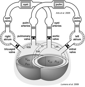
• Arts et al. (2005): https://doi.org/10.1152/ajpheart.00444.2004

• Lumens et al. (2009): https://doi.org/10.1007/s10439-009-9774-2

• Walmsley et al. (2015): https://doi.org/10.1371/journal.pcbi.1004284

Basics of Python

Always start the document with importing modules. Numpy is used for mathematics, Matplotlib for plots and are conventionally imported as np and plt respectively. Also import the CircAdapt model in this section.

import numpy as np
import matplotlib.pyplot as plt
import circadapt

Parameters types are automatically set or changed by the interpreter, but it is good to create an integer when you need an integer and float when needed.

i = 1                 # integer
f = 1.                # float
b = True              # bool
l = [1, 2, 3]         # list
d = {'a': 1, 'b': 2}  # dictionary

# get data from the list and dictionary
first_item_of_list = l[0]
item_from_dictionary = d['a']

print('First item of list = ', first_item_of_list)
print('Item from dictionary = ', item_from_dictionary)

# the use of numpy is advised for more complex use and for calculation
numpy_array = np.array(l)
print('Find if array is 2: ', (numpy_array == 2))
print('Multiply array with 2: ', (numpy_array * 2))

First item of list =  1
Item from dictionary =  1
Find if array is 2:  [False  True False]
Multiply array with 2:  [2 4 6]

You can also press f9 to run a single line or selection and press crtl+enter to run a block seperated by #%%

Load the model

# Only import the class we need in this tutorial.
from circadapt import VanOsta2024

model = VanOsta2024()

The model consists of different modules representing the atrial and ventricular cavities, with intraventricular septum, atrioventricular and ventriculoarterial valves, major blood vessels, both pulmonary and systemic vasculature and the pericardium.

To see which exact modules the model contains, these can be printed in the (ipython) console with the following code:

# model components can be retrieved as a list of strings
components = model.components
print('Components of this model: \n', components)

Components of this model: 
 ['ArtVen', 'Bag', 'Cavity', 'Chamber', 'Connector', 'General', 'Node', 'PFC', 'Patch', 'Solver', 'Timings', 'TriSeg', 'Tube0D', 'Valve', 'Wall']

Each component may contain

1. Parameters

   these values can be changed according to the pathology you are interested in

2. Signals

   these are the resulting signals after the model has simulated a heartbeat, which can be retrieved from the model

3. Objects

   here, the objects are listed to which the parameters and signals correspond, i.e. the first value of a parameter corresponds to the first object

Let’s take the Valve component as an example. To access the Valve, we use the following code:

# Access the Valve component and show the parameters, signals and objects for this component

print('The Valve component contains the following: \n', model['Valve'])

The Valve component contains the following: 
 <AutoComponent> 
parameters: 
 ['A_leak', 'A_open', 'L_fac_dist', 'L_fac_prox', 'L_fac_valve', 'adaptation_A_open_fac', 'fraction_A_open_Aext', 'l', 'p0_closure', 'papillary_muscles_A_open_fac', 'papillary_muscles_min', 'papillary_muscles_slope', 'q', 'rho_b', 'scaleQ', 'papillary_muscles', 'soft_closure']

 signals: 
 ['q', 'L', 'A', 'Dp', 'DpB', 'L', 'dq_dt', 'diast']

 objects: 
 ['Model.Peri.SyVenRa', 'Model.Peri.RaRv', 'Model.Peri.RvPuArt', 'Model.Peri.PuVenLa', 'Model.Peri.LaLv', 'Model.Peri.LvSyArt']
<\AutoComponent>

We now want to see the effective orifice areas (parameter A_open) for each object. The values for this parameter then correspond to the different objects (valves) that this module contains:

# We can obtain all orifice areas 
print('Effective orifice areas for each valve: \n', model['Valve']['A_open'], '\n')

# or we can obtain a specific orifice area, for example the aortic valve (object 'LvSyArt' --> valve between the LV and the systemic arteries)
print('Effective orifice area for the aortic valve: \n', model['Valve']['A_open']['LvSyArt'], '\n')

print('Note that the aortic valve (6th object) corresponds to the 6th position within A_open')

Effective orifice areas for each valve: 
 array([0.00049916, 0.00047155, 0.00047155, 0.00050805, 0.00049835,
       0.00049835]) 

Effective orifice area for the aortic valve: 
 0.00049835 

Note that the aortic valve (6th object) corresponds to the 6th position within A_open

Hemodynamic signals are not stored when the CircAdapt model is imported, so they are only available after running a beat.

Therefore, the model should run. You can either run a number of beats, or run until the model is hemodynamically stable.

model.run(5)
model.run(stable=True)

Plot global hemodynamics

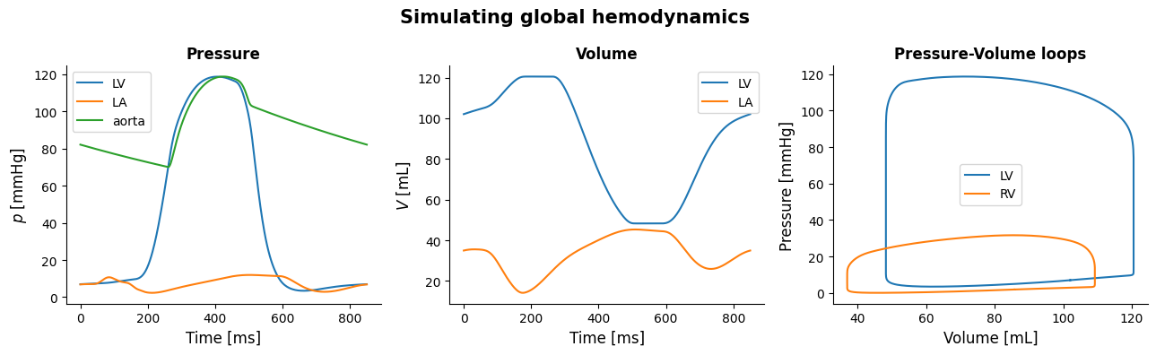
Here is an example code to plot pressures, volumes and pressure-volume loops.

First we retrieve the hemodynamic signals that we are interested in, those are:

• Pressures of the LV, LA, aorta and RV

• Volumes of the LV, LA and RV

• Time

We can obtain pressures and volumes from the Cavity component. Since were are interested in the hemodynamic signals, we access these by entering the component, followed by the signal and cavity of interest:

model[‘Cavity’][‘signal of interest’][:, ‘cavity of interest’]

Here, we use ‘:’ followed by the cavity of interest, since the hemodynamic signals are traces over time.

We obtain the pressures and volumes from the Cavity component and the time from the Solver component, and assign them to a variable according to the synthax as used above:

# get volume and pressure of LV
V_lv = model['Cavity']['V'][:, 'cLv']*1e6
p_lv = model['Cavity']['p'][:, 'cLv']*7.5e-3

# get volume and pressure of LA
V_la = model['Cavity']['V'][:, 'La']*1e6
p_la = model['Cavity']['p'][:, 'La']*7.5e-3

# get volume and pressure of RV
V_rv = model['Cavity']['V'][:, 'cRv']*1e6
p_rv = model['Cavity']['p'][:, 'cRv']*7.5e-3

# get aortic pressure
p_ao = model['Cavity']['p'][:, 'SyArt']*7.5e-3

# get time
time = model['Solver']['t']*1e3

# if in doubt about the exact naming of the cavity objects, use:
print('Check exact names of the objects: \n', model['Cavity'].objects)

Check exact names of the objects: 
 ['Model.SyArt', 'Model.SyVen', 'Model.PuArt', 'Model.PuVen', 'Model.Peri', 'Model.Peri.La', 'Model.Peri.Ra', 'Model.Peri.TriSeg.cLv', 'Model.Peri.TriSeg.cRv']

# you can also obtain multiple signals at the same time, after which you can split the two pressure signals into two parameters 
# using the following lines. First transpose the pressure such that the first axis sets the signals

pressure = model['Cavity']['p'][:, ['cLv', 'cRv']]*7.5e-3
p_lv, p_rv = pressure.T

Now that we have obtained all signals, we open a figure and add three different subplots to it. Assigning this figure to a variable is optional, but is useful for design purposes.

# Plot data
fig = plt.figure(1, figsize=(13, 4))
ax1 = fig.add_subplot(1, 3, 1)
ax2 = fig.add_subplot(1, 3, 2)
ax3 = fig.add_subplot(1, 3, 3)

# Plot pressures
ax1.plot(time, p_lv, label = 'LV')
ax1.plot(time, p_la, label = 'LA')
ax1.plot(time, p_ao, label = 'aorta')
ax1.legend()

# Plot volumes
ax2.plot(time, V_lv, label = 'LV')
ax2.plot(time, V_la, label = 'LA')
ax2.legend()

# Plot PV loops
ax3.plot(V_lv, p_lv, label = 'LV')
ax3.plot(V_rv, p_rv, label = 'RV')
ax3.legend()

# plot design, add labels
for ax in [ax1, ax2, ax3]:
    ax.spines[['right', 'top']].set_visible(False)
ax1.set_xlabel('Time [ms]', fontsize=12)
ax2.set_xlabel('Time [ms]', fontsize=12)
ax3.set_xlabel('Volume [mL]', fontsize=12)

ax1.set_ylabel('$p$ [mmHg]', fontsize=12)
ax2.set_ylabel('$V$ [mL]', fontsize=12)
ax3.set_ylabel('Pressure [mmHg]', fontsize=12)

ax1.set_title('Pressure',
             fontsize=12, fontweight='bold')
ax2.set_title('Volume',
             fontsize=12, fontweight='bold')
ax3.set_title('Pressure-Volume loops',
             fontsize=12, fontweight='bold')

fig.suptitle('Simulating global hemodynamics ',
             fontsize=15, fontweight='bold')

plt.tight_layout()
plt.draw()

Save and load the model

# Use .npy extension in filename to save the model
model.save('reference.npy')

# First import the reference model after which you load the previously saved model
loaded_model = VanOsta2024()
loaded_model.load('reference.npy')

# If you want to save and load a structure without writing it to a file, use the follow lines. 
# Note that signals are not filled, you have to run at least 1 beat

data = model.model_export()
model.model_import(data)