Tutorial VanOsta2024

.. tags:: ArtVen, Bag, Chamber2022, TriSeg2022, Valve2022, Timings, PressureFlowControl

The goal of this tutorial is to understand the CircAdapt framework and to use the VanOsta2022 model. This tutorial assumes little to no knowledge about python. Therefore, basic python conventions and syntax will be discussed.

This tutorial will use matplotlib.pyplot for visualizations and numpy for mathematical operations. It is common to import it using:

import matplotlib.pyplot as plt
import numpy as np

In this tutorial, we will use the built-in model VanOsta2024. Import the model and create a model object.

from circadapt import VanOsta2024
model = VanOsta2024()

CircAdapt tries to follow the syntax of python and numpy as much as possible. The object can be handled as a dictionary. Content can be printed in the console, and printed on request in the ipython console.

model

<VanOsta2024>
CircAdapt object with keys:
['ArtVen', 'Bag', 'Cavity', 'Chamber', 'Connector', 'General', 'Node', 'PFC', 'Patch', 'Solver', 'Timings', 'TriSeg', 'Tube0D', 'Valve', 'Wall']
<\VanOsta2024>

Components can also be retrieved as a list of strings.

components = model.components
print('Components of this model: ', components, '\n')

Components of this model:  ['ArtVen', 'Bag', 'Cavity', 'Chamber', 'Connector', 'General', 'Node', 'PFC', 'Patch', 'Solver', 'Timings', 'TriSeg', 'Tube0D', 'Valve', 'Wall'] 

Similar to the object itself, components can be printed

model['Patch']

<Patch> 
parameters: 
 ['Am_ref', 'V_wall', 'v_max', 'l_se0', 'l_s0', 'l_s_ref', 'dl_s_pas', 'Sf_pas', 'ft1_const', 'tr', 'td', 'time_act', 'Sf_act', 'fac_Sf_tit', 'k1', 'dt', 'C_rest', 'l_si0', 'LDAD', 'ADO', 'LDCC', 'SfPasMaxT', 'SfPasActT', 'FacSfActT', 'LsPasActT', 'adapt_gamma', 'transmat00', 'transmat01', 'transmat02', 'transmat03', 'transmat10', 'transmat11', 'transmat12', 'transmat13', 'transmat20', 'transmat21', 'transmat22', 'transmat23']

 signals: 
 ['l_s', 'l_si', 'l_si_dot', 'C', 'C_dot', 'Cm', 'Am', 'Am0', 'Ef', 'dA_dT', 'Sf', 'Sf_pas_total', 'Sf_ecm', 'dSf_dEf', 'dSf_pas_dEf', 'SfEcmMax', 'SfActMax', 'SfPasAct', 'LsPasAct', 'moment_of_activation']

 objects: 
 ['Model.Peri.La.wLa.pLa0', 'Model.Peri.Ra.wRa.pRa0', 'Model.Peri.TriSeg.wLv.pLv0', 'Model.Peri.TriSeg.wSv.pSv0', 'Model.Peri.TriSeg.wRv.pRv0']
<\Patch>

Each component points to multiple c++ objects of that component type. The objects can also be obtained using

objects = model['Patch'].objects
parameters = model['Patch'].parameters
signals = model['Patch'].signals

Signals are not stored, so they are only available after running a beat. Therefore the model should run. You can either run a number of beats, or run until the model is hemodynamically stable.

model.run(5)
model.run(stable=True)

Plot global hemodynamics

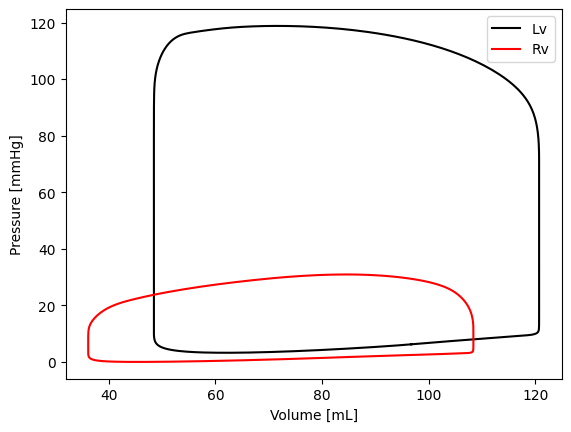
Here is an example code to plot the PV loop First we open a figure. Assigning this figure to a variable is optional, but is useful for design purposes.

fig = plt.figure(1)

# get volume and pressure of LV
Vlv = model['Cavity']['V'][:, 'cLv']*1e6
plv = model['Cavity']['p'][:, 'cLv']*7.5e-3

# get volume and pressure of RV
Vrv = model['Cavity']['V'][:, 'cRv']*1e6
prv = model['Cavity']['p'][:, 'cRv']*7.5e-3

# You can also use location names to get/set signals and parameters
# For this, use only the last part of the full object name, e.g. cLv for
# Model.Peri.TriSeg.cLv. You can get one signal or multiple signals
Vlv = model['Cavity']['V'][:, 'cLv']*1e6
Vrv = model['Cavity']['V'][:, 'cRv']*1e6
pressure = model['Cavity']['p'][:, ['cLv', 'cRv']]*7.5e-3

# you can split the two pressure signals into two parameters using the
# following line. First transpose the pressure such that the first axis sets
# the signals
plv, prv = pressure.T

# Now we plot the two lines.
line1 = plt.plot(Vlv, plv, c='k', label='Lv')
line2 = plt.plot(Vrv, prv, c='r', label='Rv')
plt.ylabel('Pressure [mmHg]')
plt.xlabel('Volume [mL]')
plt.legend()

<matplotlib.legend.Legend at 0x29a58960c20>

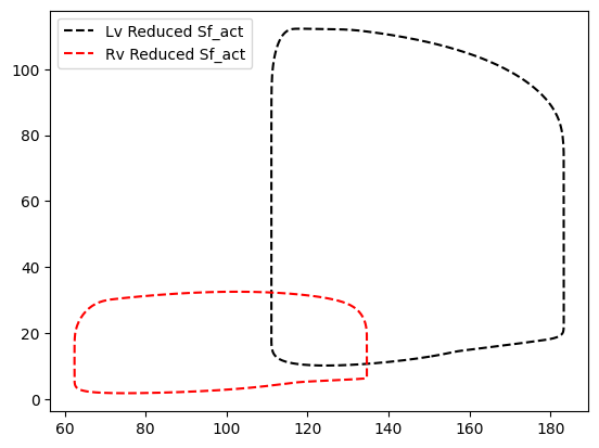
Change parameters

# Now reduce the contractility of all 3 ventricular walls
model['Patch']['Sf_act'][2:] = 60e3

# We can also explicitly change the ventricular wall patches
model['Patch']['Sf_act'][['pLv0', 'pSv0', 'pRv0']] = 60e3

# or do it one by one
model['Patch']['Sf_act']['pLv0'] = 60e3
model['Patch']['Sf_act']['pSv0'] = 60e3
model['Patch']['Sf_act']['pRv0'] = 60e3

# run the simulation and plot
model.run(stable=True)
plt.plot(model['Cavity']['V'][:, 'cLv']*1e6, model['Cavity']['p'][:, 'cLv']*7.5e-3, 'k--', label='Lv Reduced Sf_act')
plt.plot(model['Cavity']['V'][:, 'cRv']*1e6, model['Cavity']['p'][:, 'cRv']*7.5e-3, 'r--', label='Rv Reduced Sf_act')
plt.legend()

<matplotlib.legend.Legend at 0x29a7f32f4a0>

Multipatch and local dynamics

# Set up a new multipatch model and set an activation delay
model_multipatch = VanOsta2024()

# The number of patches is specified in the wall. Here, we set 12 Lv patches
# and 6 Sv patches. Then, we change the dt in these patches.
model_multipatch['Wall']['n_patch'][2:4] = [12, 6]
model_multipatch['Patch']['dt'][2:14] = np.linspace(0, 0.01, 12)
model_multipatch['Patch']['dt'][14:20] = np.linspace(0, 0.01, 6)

# Run beats
model_multipatch.run(stable=True)

# Plot data
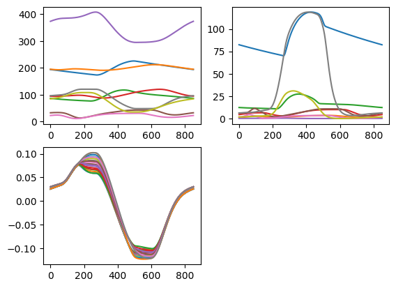
fig = plt.figure(2)

# In the first subplot, plot all volumes
ax1 = plt.subplot(2, 2, 1)
plt.plot(model_multipatch['Solver']['t']*1e3,
         model_multipatch['Cavity']['V']*1e6,
         )
# in the second subplot, plot all pressures
ax1 = plt.subplot(2, 2, 2)
plt.plot(model_multipatch['Solver']['t']*1e3,
         model_multipatch['Cavity']['p']*7.5e-3,
         )
# in the third subplot, plot all natural fiber strains.
ax1 = plt.subplot(2, 2, 3)
plt.plot(model_multipatch['Solver']['t']*1e3,
         model_multipatch['Patch']['Ef'][:, 2:20],
         )

# %% 6. Save and Load
# Simulations can be saved and loaded using the following code.
model_reference = VanOsta2024()

# use .npy extension in filename
model_reference.save('reference.npy')

# ander bestand
model = VanOsta2024()
model.load('reference.npy')

# if you want to save and load a structure without writing it to a file, use
# the follow lines. Note that signals are not filled, you have to run at least
# 1 beat.
data = model_reference.model_export()
model_reference.model_import(data)