VanOsta2024

Model summary

Cheatsheet

Tutorials

circadapt.VanOsta2024([solver, ...])

The VanOsta2024 model was initially introduced by van Osta et al.[1]. It is founded on the CircAdapt model published by Walmsley in 2015 Walmsley et al.[2]. On this page, a general description is given on the model. Tutorials for this model can be found here.

Physiological Background

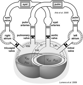
In a normal adult, the heart has four chambers, the left and right atrium and the left and right ventricle. Two valves connect the atria with the ventricles. The tricuspid valve is positioned between the right atrium and the right ventricle, and the mitral valve between the left atrium and the left ventricle. Besides these atrio-ventricular inlet valves, each ventricle has a ventricular-arterial outlet valve connecting them to the systemic and pulmonary circulation. The pulmonary valve lies between the right ventricle and the pulmonary artery, and the aortic valve lies between the left ventricle and the aorta. Wall strain determines the wall tension resulting from the passive and active material behavior of the myocardial tissue. Wall tension together with geometry determine the cavity pressure.

The pressure in a heart chamber is determined by the cavity volume. The cavity volume determines the myofibers strain. Myofiber stress arises from myofiber strain. The myofibers have a well-documented helical arrangement in the ventricles (Streeter Jr et al.[3]), and have a considerably more complex arrangement in the atria (Ho and Sanchez-Quintana[4]). Besides, the myofibers are loosely arranged into sheet-like structures. Myofiber stress is a summation of active stress, generated by the sarcomere, and passive stress resulting from stretch of elastic structures, primarily attributed to the extracellular matrix (ECM). The stress-strain relationship of the myocardial tissue is discussed in more detail in the documentation for the sarcomere module. The atria may be considered as simple cavities, encapsulated each by a relatively thin contractile elastic wall. In the CircAdapt model (Arts et al.[5], Lumens et al.[6]), each atrium is simulated by a Chamber-module. The ventricular unit is more complicated, because the right and left ventricle interact by their shared wall, the septum (Lumens et al.[6], Lumens et al.[7]). In the CircAdapt model, the composition of the left and right ventricle is simulated by a TriSegmodule. Mechanical interaction of the atrial walls with each other and with the ventricular walls probably occurs in the human heart, but is neglected because these interactions are relatively insignificant (Goldstein et al.[8], Henein et al.[9]).

In many examples of cardiac pathology, mechanical properties are inhomogeneously distributed over the various walls. To simulate such inhomogeneities in CircAdapt, the wall has been subdivided in a number of patches, each having specific mechanical properties. A patch is modeled by a Patch-module, allowing to have specific timing of activation, specific contractile properties and specific passive elastic properties. The Wall links the Patch mechanics to global hemodynamics.

Model Description

This model represents a rapid biomechanical lumped-parameter approach to simulate the intricacies of the heart and circulatory system. It uses a one-fiber model (Chamber and Wall) to establish the wall stress and cavity pressure relationship. The TriSeg module facilitates inter-ventricular interaction across the Intra-Ventricular Septum (IVS) (TriSeg). Phenomenological material laws define the active and passive stress–strain relationship in the spherical walls (Patch). The MultiPatch module introduces regional heterogeneity of tissue properties within a single wall (Wall).

Additionally, a reduced-order circulation is implemented, with systemic and pulmonary arteries and veins modeled using a single Tube0D each. The flow across systemic and pulmonary capillaries is simulated using the ArtVen module. Flow from atria to ventricles, from ventricles to arteries, and from veins to atria are simulated by means of the Valve module.

At a global scale, the Timings module manages atrial and ventricular activation. Homeostatic control can be regulated through PressureFlowControl when activated.

Default parameterization

The model is initiated with a default parameterization which represents healthy physiology. This can be visualized using the default plot statement as shown below and can be generated using the following code:

import circadapt
import matplotlib.pyplot as plt

model = circadapt.VanOsta2024()
model.run(stable=True)
model.plot()
plt.show()

(Source code, png, hires.png, pdf)

Fig. 18 Default visualization of the model with its reference parameterization.

This default parameterization gives the following scalar output:

Table 1 Model compared to reference values

	Model	Literature	Unit	Source
LVEDV	120.6	121 pm 31	mL	Addetia et al.[10]
LVESV	48.3	47 pm 15	mL	Addetia et al.[10]
LVEF	59.9	61 pm 5	%	Addetia et al.[10]
RVEDV	108.2	91 [61 - 150]	mL	Maffessanti et al.[11]
RVESV	35.9	35 [16 - 72]	mL	Maffessanti et al.[11]
RVEF	66.8	62 [47 - 77]	%	Maffessanti et al.[11]
SBP	119.1	121 pm 12	mmHg	Addetia et al.[10]
DBP	70.3	74 pm 9	mmHg	Addetia et al.[10]
mPAP	16.1	[8 - 20]	mmHg	Humbert et al.[12]
mLAP	6.5	0 - 15	mmHg	Humbert et al.[12]
mRAP	1.9	2 - 6	mmHg	Humbert et al.[12]

Model assumptions and parameterizations

Todo

• Explain the solving strategy.

• Present the initial parameterization.

• Discuss the model verification process.

• Explain adaptation protocol

Solving strategy

Todo

Update overview of the framework and its solving strategy.

Each object in this model is derived from one of the CircAdapt modules. An overview of all these objects is shown in below. All Modules together form the ordinary differential equations, which are solved using one of the implemented Solvers. By default, this set is solved using a Adams Moulton solver with a time stepsize of 0.001ms.

(Source code)

References

[1]

Nick van Osta et al. Under review. ():, 2024. URL:.

[2]

John Walmsley, Theo Arts, Nicolas Derval, Pierre Bordachar, Hubert Cochet, Sylvain Ploux, Frits W. Prinzen, Tammo Delhaas, and Joost Lumens. Fast simulation of mechanical heterogeneity in the electrically asynchronous heart using the multipatch module. PLOS Computational Biology, 11(7):1–23, 07 2015. URL: https://doi.org/10.1371/journal.pcbi.1004284, doi:10.1371/journal.pcbi.1004284.

[3]

Daniel D Streeter Jr, Henry M Spotnitz, Dali P Patel, John Ross Jr, and Edmund H Sonnenblick. Fiber orientation in the canine left ventricle during diastole and systole. Circulation research, 24(3):339–347, 1969.

[4]

SY Ho and D Sanchez-Quintana. The importance of atrial structure and fibers. Clinical Anatomy: The Official Journal of the American Association of Clinical Anatomists and the British Association of Clinical Anatomists, 22(1):52–63, 2009.

[5]

Theo Arts, Tammo Delhaas, Peter Bovendeerd, Xander Verbeek, and Frits W Prinzen. Adaptation to mechanical load determines shape and properties of heart and circulation: the circadapt model. American Journal of Physiology-Heart and Circulatory Physiology, 288(4):H1943–H1954, 2005.

[6] (1,2)

Joost Lumens, Tammo Delhaas, Borut Kirn, and Theo Arts. Three-wall segment (triseg) model describing mechanics and hemodynamics of ventricular interaction. Annals of biomedical engineering, 37:2234–2255, 2009.

[7]

Joost Lumens, Sylvain Ploux, Marc Strik, John Gorcsan, Hubert Cochet, Nicolas Derval, Maria Strom, Charu Ramanathan, Philippe Ritter, Michel Haïssaguerre, and others. Comparative electromechanical and hemodynamic effects of left ventricular and biventricular pacing in dyssynchronous heart failure: electrical resynchronization versus left–right ventricular interaction. Journal of the American College of Cardiology, 62(25):2395–2403, 2013.

[8]

James A Goldstein, James S Tweddell, Benico Barzilai, Yoko Yagi, Allan S Jaffe, and James L Cox. Hemodynamic effects of atrial interaction. Coronary Artery Disease, 4(6):545–553, 1993.

[9]

Mark Henein, Yat-Yin Lam, Anders Waldenstöm, and Michael Y Henein. Atrial interaction in the form of ‘cross talk’in patients with ventricular outflow tract obstruction. International journal of cardiology, 147(3):388–392, 2011.

[10] (1,2,3,4,5)

Karima Addetia, Tatsuya Miyoshi, Vivekanandan Amuthan, Rodolfo Citro, Masao Daimon, Pedro Gutierrez Fajardo, Ravi R Kasliwal, James N Kirkpatrick, Mark J Monaghan, Denisa Muraru, and others. Normal values of left ventricular size and function on three-dimensional echocardiography: results of the world alliance societies of echocardiography study. Journal of the American Society of Echocardiography, 35(5):449–459, 2022.

[11] (1,2,3)

Francesco Maffessanti, Denisa Muraru, Roberta Esposito, Paola Gripari, Davide Ermacora, Ciro Santoro, Gloria Tamborini, Maurizio Galderisi, Mauro Pepi, and Luigi P Badano. Age-, body size-, and sex-specific reference values for right ventricular volumes and ejection fraction by three-dimensional echocardiography: a multicenter echocardiographic study in 507 healthy volunteers. Circulation: Cardiovascular Imaging, 6(5):700–710, 2013.

[12] (1,2,3)

Marc Humbert, Gabor Kovacs, Marius M Hoeper, Roberto Badagliacca, Rolf MF Berger, Margarita Brida, Jørn Carlsen, Andrew JS Coats, Pilar Escribano-Subias, Pisana Ferrari, and others. 2022 esc/ers guidelines for the diagnosis and treatment of pulmonary hypertension: developed by the task force for the diagnosis and treatment of pulmonary hypertension of the european society of cardiology (esc) and the european respiratory society (ers). endorsed by the international society for heart and lung transplantation (ishlt) and the european reference network on rare respiratory diseases (ern-lung). European heart journal, 43(38):3618–3731, 2022.

Python implementation

class circadapt.VanOsta2024(solver: str = None, path_to_circadapt: str = None, model_state: dict = None)

Bases: Model, ModelAdapt

adapt(options: dict = {}, output: bool = False, verbose: bool = False) → None

Run adaptation protocol.

The adaptation protocol runs n_cycles cycles. Each cycle has two phases, namely rest adaptation and exercise adaptation. First, in exercise, the Patches and vessel wall volumes are adapted to load. In rest, vessels are adapted to flow.

Parameters

optionsdictionary, optional

Options for the protocol. To set options, use the function get_adapt_options(), which is used by default. The default is {}.

outputbool, optional

DESCRIPTION. The default is False.

Returns

senses_resultsTYPE

Only when output=True.

senses_normTYPE

Only when output=True.

actor_resultsTYPE

Only when output=True.

actor_vwallTYPE

Only when output=True.

adapt_exercise(options)

Trigger all excercise adaptation functions.

adapt_rest(options)

Trigger all rest adaptation functions.

add(comp_type: str) → bool

add_component(comp_type: str, comp_name: str, base: str = '') → bool

Add component to CircAdapt object.

Parameters

comp_type: str

Type of object to create in the ComponentFactory

comp_name: str

Name of the new object to create

base: char, optional (default=’’)

Parent object of new component

Returns

is_success (bool)

add_smart_component(smart_component, base=None, **kwargs)

assert_1_beat()

Test status after 1 beat, used in unit tests.

build()

Build model.

Add and link components in the model. By default, the model is empty. This function will be used in derived model builts.

build_artven(base=None, **kwargs)

build_heart(base=None, options=None)

build_pfc(base=None, options=None)

build_timings(base=None, options=None)

calculate_and_set_matrix(verbose=False)

check_build()

copy()

Return a copy of itself.

get(*arg, **kwarg)

get_adapt_options()

Get default adapt options.

get_matrix(verbose=False)

get_model_reference(model_state: any = None) → dict

Return reference model state as a dictionary.

If model_state is string, it is assumed to be a file location. This file will be loaded and returned. If is none, the default reference will be loaded. If no default reference available, it will be created and stored in the current active directory.

Parameters

model_statestr or None, optional

Location of model state. The default is None.

Raises

ValueError

DESCRIPTION.

Returns

dict

Dictonary with model state.

get_unittest_results(model)

Real-time results after initializing and running 1 beat.

get_unittest_targets()

Hardcoded results after initializing and running 1 beat.

health_check()

Manually perform tests to check compatibility of model with version.

install()

is_stable() → bool

Check if simulation is hemodynamically stable.

is_success() → bool

Return false if vectors contain nan.

Returns

bool

load(filename: str) → None

Load a model dataset from a filename.

Parameters

filename: str

Path to file that will be loaded. The extension must be .npy or .mat.

load_plugin_components(path_to_library: str)

Load a plugin

Parameters

path_to_librarystr

Path to library.

load_reference()

Load reference of current model from the package.

model_export(style: str = None) → dict

Return the stored model state.

Parameters

style: str (optional)

Style to follow. If not given, the default style from the model is used.

Returns

dict

model_import(model_state, check_model_state=False) → None

Load model_state into CircAdapt object.

Style and model_state version is automatically recognized.

Parameters

model_state: dict

model_state with data to set

obj: str

Object to set

plot(fig=None)

Simple plot to illustrate the model state.

plot_extended(fig=None)

Extended plot to illustrate the model state.

run(*arg, **kwarg)

save(filename: str, ext: str = None) → None

Save model to filename with extention.

Parameters

filename: str

Filename to save file to. Filename must have extention .npy or .mat

ext: str (optional)

Extention of the file. If not given, the last 3 letters of the filename is used to determine the save method.

set(*arg, **kwarg)

set_component(par, *arg, **kwarg)

set_reference()

trigger(par) → bool

Trigger a function.

Objects in the model may have a function that can be triggered. This can be done by triggering the function using the ‘par’ parameter similar to the set function, only without a parameter.

Parameters

parstr

Function in object that will be triggered. It has a similar form to the set/get par, i.e. ‘Component.subcomponent.function_name’

Returns

is_success (bool)

class VanOsta2024(Model, ModelAdapt):
    def __init__(self,
                 solver: str = None,
                 path_to_circadapt: str = None,
                 model_state: dict = None,
                 ):
        if solver is None:
            solver = 'adams_moulton'

        self._local_save_reference = True

        ModelAdapt.__init__(self)
        Model.__init__(self,
                       solver,
                       path_to_circadapt=path_to_circadapt,
                       model_state=model_state,
                       )

    def _update_settings(self):
        # rename model components for easy input/output
        self._module_rename['PressureFlowControl'] = 'PFC'

    def build(self):
        pass
        # Circulation
        self.add_smart_component('ArtVen', build='SystemicCirculation')
        self.add_smart_component('ArtVen', build='PulmonaryCirculation')
        self.add_smart_component('Heart', patch_type='Patch', valve_type='Valve')
        self.add_smart_component('Timings')
        self.add_smart_component('PressureFlowControl')

        self.set_component('PFC.circulation_volume_object', 'SyArt')
        self.set_component('PFC.circulation_volume_object', 'SyVen')
        self.set_component('PFC.circulation_volume_object', 'PuArt')
        self.set_component('PFC.circulation_volume_object', 'PuVen')
        self.set_component('PFC.circulation_volume_object', 'Peri.La')
        self.set_component('PFC.circulation_volume_object', 'Peri.Ra')
        self.set_component('PFC.circulation_volume_object', 'Peri.TriSeg.cLv')
        self.set_component('PFC.circulation_volume_object', 'Peri.TriSeg.cRv')

        # # manually set papillary muscles
        self.set_component("Peri.RaRv.wPapMus", "Peri.TriSeg.wRv")
        self.set_component("Peri.LaLv.wPapMus", "Peri.TriSeg.wLv")

    def set_reference(self):
        self['Chamber']['buckling'] = True
        self['Valve']['soft_closure'] = True
        self['Valve']['papillary_muscles'] = False

        self['Solver']['dt'] = 0.001
        self['Solver']['dt_export'] = 0.002
        self.set('Solver.order',  2)

        self.set('Model.t_cycle', 0.85)
        self['ArtVen']['p0'] = np.array([6306.25832487, 1000.        ])
        self['ArtVen']['q0'] = np.array([4.5e-05, 4.5e-05])
        self['ArtVen']['k'] = np.array([1., 2.])
        self['Tube0D']['l'] = np.array([0.4, 0.4, 0.2, 0.2])
        self['Tube0D']['A_wall'] = np.array([1.12362733e-04, 6.57883944e-05, 9.45910889e-05, 8.22655361e-05])
        self['Tube0D']['k'] = np.array([1.66666667, 2.33333333, 1.66666667, 2.33333333])
        self['Tube0D']['p0'] = np.array([12162.50457811,   287.7083132 ,  2132.51755623,   830.54673184])
        self['Tube0D']['A0'] = np.array([0.0004983 , 0.00049909, 0.00047138, 0.00050803])
        self['Tube0D']['target_wall_stress'] = np.array([500000., 500000., 500000., 500000.])
        self['Tube0D']['target_mean_flow'] = np.array([0.17, 0.17, 0.17, 0.17])
        self['Bag']['k'] = np.array([10.])
        self['Bag']['p_ref'] = np.array([1000.])
        self['Bag']['V_ref'] = np.array([0.00054267])
        self['Patch']['Am_ref'] = np.array([0.00425687, 0.00401573, 0.00966859, 0.00289936, 0.01084227])
        self['Patch']['V_wall'] = np.array([4.46069398e-06, 2.14548521e-06, 7.35720515e-05, 1.88904978e-05, 3.67720116e-05,])
        self['Patch']['v_max'] = np.array([14., 14.,  7.,  7.,  7.])
        self['Patch']['l_se0'] = np.array([0.04, 0.04, 0.04, 0.04, 0.04])
        self['Patch']['l_s0'] = np.array([1.8, 1.8, 1.8, 1.8, 1.8])
        self['Patch']['l_s_ref'] = np.array([2., 2., 2., 2., 2.])
        self['Patch']['dl_s_pas'] = np.array([0.6, 0.6, 0.6, 0.6, 0.6])
        self['Patch']['Sf_pas'] = np.array([2248.53598   , 2684.76100348,  731.24545453,  729.06063771, 749.47694522,])
        self['Patch']['tr'] = np.array([0.4 , 0.4 , 0.25, 0.25, 0.25])
        self['Patch']['td'] = np.array([0.4 , 0.4 , 0.25, 0.25, 0.25])
        self['Patch']['time_act'] = np.array([0.15 , 0.15 , 0.425, 0.425, 0.425])
        self['Patch']['Sf_act'] = np.array([ 84000.,  84000., 120000., 120000., 120000.])
        self['Patch']['fac_Sf_tit'] = np.array([0.01, 0.01, 0.01, 0.01, 0.01])
        self['Patch']['k1'] = np.array([10., 10., 10., 10., 10.])
        self['Patch']['dt'] = np.array([0., 0., 0., 0., 0.])
        self['Patch']['C_rest'] = np.array([0., 0., 0., 0., 0.])
        self['Patch']['l_si0'] = np.array([1.51, 1.51, 1.51, 1.51, 1.51])
        self['Patch']['LDAD'] = np.array([1.057, 1.057, 1.057, 1.057, 1.057])
        self['Patch']['ADO'] = np.array([0.65, 0.65, 0.65, 0.65, 0.65])
        self['Patch']['LDCC'] = np.array([4., 4., 4., 4., 4.])
        self['Patch']['SfPasMaxT'] = np.array([320000., 320000.,  16000.,  16000.,  16000.])
        self['Patch']['SfPasActT'] = np.array([40000., 40000., 20000., 20000., 20000.])
        self['Patch']['FacSfActT'] = np.array([0.8, 0.8, 1. , 1. , 1. ])
        self['Patch']['LsPasActT'] = np.array([2.42, 2.42, 2.42, 2.42, 2.42])
        self['Patch']['adapt_gamma'] = np.array([0.5, 0.5, 0.5, 0.5, 0.5])
        self['Patch']['transmat00'] = np.array([-0.5751, -0.5751, -0.5751, -0.5751, -0.5751])
        self['Patch']['transmat01'] = np.array([-0.7851, -0.7851, -0.7851, -0.7851, -0.7851])
        self['Patch']['transmat02'] = np.array([0.6063, 0.6063, 0.6063, 0.6063, 0.6063])
        self['Patch']['transmat03'] = np.array([-0.5565, -0.5565, -0.5565, -0.5565, -0.5565])
        self['Patch']['transmat10'] = np.array([-0.1279, -0.1279, -0.1279, -0.1279, -0.1279])
        self['Patch']['transmat11'] = np.array([0.0999, 0.0999, 0.0999, 0.0999, 0.0999])
        self['Patch']['transmat12'] = np.array([0.2066, 0.2066, 0.2066, 0.2066, 0.2066])
        self['Patch']['transmat13'] = np.array([-1.8441, -1.8441, -1.8441, -1.8441, -1.8441])
        self['Patch']['transmat20'] = np.array([-0.1865, -0.1865, -0.1865, -0.1865, -0.1865])
        self['Patch']['transmat21'] = np.array([-0.201, -0.201, -0.201, -0.201, -0.201])
        self['Patch']['transmat22'] = np.array([1.3195, 1.3195, 1.3195, 1.3195, 1.3195])
        self['Patch']['transmat23'] = np.array([-11.8745, -11.8745, -11.8745, -11.8745, -11.8745])
        self['Valve']['adaptation_A_open_fac'] = np.array([1., 1., 1., 1., 1., 1.])
        self['Valve']['A_open'] = np.array([0.00049916, 0.00047155, 0.00047155, 0.00050805, 0.00049835,
               0.00049835])
        self['Valve']['A_leak'] = np.array([0.00049916, 1.e-09, 1.e-09, 0.00050805, 1.e-09, 1.e-09])
        self['Valve']['l'] = np.array([0.01260512, 0.01225144, 0.01225144, 0.01271679, 0.01259479,
               0.01259479])
        self['Valve']['L_fac_prox'] = np.array([0.75, 0.75, 0.75, 0.75, 0.75, 0.75])
        self['Valve']['L_fac_dist'] = np.array([0.75, 0.75, 0.75, 0.75, 0.75, 0.75])
        self['Valve']['L_fac_valve'] = np.array([1.5, 1.5, 1.5, 1.5, 1.5, 1.5])
        self['Valve']['rho_b'] = np.array([1050., 1050., 1050., 1050., 1050., 1050.])
        self['Valve']['papillary_muscles'] = np.array([False, False, False, False, False, False])
        self['Valve']['papillary_muscles_slope'] = np.array([100., 100., 100., 100., 100., 100.])
        self['Valve']['papillary_muscles_min'] = np.array([0.1, 0.1, 0.1, 0.1, 0.1, 0.1])
        self['Valve']['papillary_muscles_A_open_fac'] = np.array([0.1, 0.1, 0.1, 0.1, 0.1, 0.1])
        self['Valve']['soft_closure'] = np.array([ True,  True,  True,  True,  True,  True])
        self['Valve']['fraction_A_open_Aext'] = np.array([0.9, 0.9, 0.9, 0.9, 0.9, 0.9])
        self['Timings']['time_fac'] = np.array([1.])
        self['Timings']['tau_av'] = np.array([0.150025])
        self['Timings']['dtau_av'] = np.array([0.])
        self['Timings']['law_tau_av'] = np.array([1])
        self['Timings']['law_Ra2La'] = np.array([1])
        self['Timings']['law_ta'] = np.array([1])
        self['Timings']['law_tv'] = np.array([1])
        self['Timings']['c_tau_av0'] = np.array([0.])
        self['Timings']['c_tau_av1'] = np.array([0.1765])
        self['Timings']['c_ta_rest'] = np.array([0.])
        self['Timings']['c_ta_tcycle'] = np.array([0.17647059])
        self['Timings']['c_tv_rest'] = np.array([0.1])
        self['Timings']['c_tv_tcycle'] = np.array([0.4])
        self['PFC']['p0'] = np.array([12200.])
        self['PFC']['q0'] = np.array([8.5e-05])
        self['PFC']['stable_threshold'] = np.array([0.0001])
        self['PFC']['is_active'] = np.array([ True])
        self['PFC']['fac'] = np.array([1.])
        self['PFC']['fac_pfc'] = np.array([1.])
        self['PFC']['epsilon'] = np.array([0.4])
        self['TriSeg']['tau'] = np.array([2.])
        self['TriSeg']['ratio_septal_LV_Am'] = np.array([0.3])
        self['TriSeg']['max_number_of_iterations'] = np.array([100.])
        self['TriSeg']['thresh_F'] = np.array([0.001])
        self['TriSeg']['thresh_dV'] = np.array([1.e-09])
        self['TriSeg']['thresh_dY'] = np.array([1.e-06])

        self.run(stable=True)
        # self.adapt()

        # set target volume
        self['PFC']['target_volume'] = self['PFC']['circulation_volume']

        return


    def get_unittest_targets(self):
        """Hardcoded results after initializing and running 1 beat."""
        return {
            'LVEDV': 120.5,
            'LVESV':  48.3,
            }

    def get_unittest_results(self, model):
        """Real-time results after initializing and running 1 beat."""
        LVEDV = np.max(model['Cavity']['V'][:, 'cLv'])*1e6
        LVESV = np.min(model['Cavity']['V'][:, 'cLv'])*1e6
        return {
            'LVEDV': LVEDV,
            'LVESV': LVESV,
            }


    def plot(self, fig=None):
        # TODO
        self.plot_extended(fig)

    def plot_extended(self, fig=None):
        if len(self['Solver']['t'])==0:
            raise RuntimeError('Can not plot the model, as no data is available. Did you simulate the model?')

        if fig is None:
            fig = 1
        if isinstance(fig, int):
            fig = plt.figure(fig, clear=True, figsize=(12, 8))

        # Settings
        grid_size = [32, 32]

        def get_lim(module, signal, locs=slice(None, None, None)):
            signal = self[module][signal][:, locs]
            lim = np.array([np.min(signal), np.max(signal)])
            lim += np.array([-1, 1]) * 0.1*np.diff(lim)
            return lim

        lim_V = get_lim('Cavity', 'V', ['cRv', 'Ra', 'La', 'cLv']) * 1e6
        lim_V[0] = 0
        lim_p = get_lim('Cavity', 'p', ['cRv', 'Ra', 'La', 'cLv']) / 133
        lim_p[0] = np.min([lim_p[0], 0])
        lim_Ls = get_lim('Patch', 'l_s')
        lim_Sf = get_lim('Patch', 'Sf') * 1e-3
        lim_q = get_lim('Valve', 'q',
                        ['LaLv', 'RaRv', 'LvSyArt', 'RaPuArt']) * 1e6

        all_lim = [lim_V, lim_p, lim_Ls, lim_Sf, lim_q]
        if (np.any(np.isnan(all_lim)) or np.any(np.isinf(all_lim))):
            lim_V = [0, 200]
            lim_p = [0, 150]
            lim_Ls = [1.5, 2.0]
            lim_Sf = [0, 100]
            lim_q = [-1e-3, 1e-3]

        # Pressure Volume plot
        axPV = plt.subplot2grid(grid_size, (0, 17), rowspan=15, colspan=15, fig=fig)
        axPV.plot(self['Cavity']['V'][:, 'cLv']*1e6,
                  self['Cavity']['p'][:, 'cLv']/133,
                  c=colors['Lv'],
                  )
        axPV.plot(self['Cavity']['V'][:, 'cRv']*1e6,
                  self['Cavity']['p'][:, 'cRv']/133,
                  c=colors['Rv'],
                  )
        axPV.plot(self['Cavity']['V'][:, 'La']*1e6,
                  self['Cavity']['p'][:, 'La']/133,
                  c=colors['La'],
                  )
        axPV.plot(self['Cavity']['V'][:, 'Ra']*1e6,
                  self['Cavity']['p'][:, 'Ra']/133,
                  c=colors['Ra'],
                  )
        axPV.spines[['top', 'right']].set_visible(False)
        axPV.set_title('Pressure-Volume loop', weight='bold')
        axPV.set_xlabel('Volume [mL]')
        axPV.set_ylabel('Pressure [mmHg]')
        axPV.spines[['bottom', 'left']].set_position(('outward', 5))

        ylabel_x_left = -0.25
        ylabel_x_right = 1.25

        # Volumes
        t = self['Solver']['t']*1e3

        axVRv = plt.subplot2grid(grid_size, (0, 0), rowspan=8, colspan=6, fig=fig)
        axVRv.plot(t, self['Cavity']['V'][:, 'cRv']*1e6,
                   c=colors['Rv'],
                   )
        axVRv.plot(t, self['Cavity']['V'][:, 'Ra']*1e6,
                   c=colors['Ra'],
                   )
        axVRv.set_ylim(lim_V)
        axVRv.set_ylabel('Volume\n[mL]')
        axVRv.spines[['top', 'right']].set_visible(False)
        axVRv.set_title('Right Heart', weight='bold')
        # axVRv.set_xticks([])
        axVRv.tick_params(axis='both', direction='in')
        axVRv.yaxis.set_label_coords(ylabel_x_left, 0.5)


        axVLv = plt.subplot2grid(grid_size, (0, 6), rowspan=8, colspan=6, fig=fig)
        axVLv.plot(t, self['Cavity']['V'][:, 'cLv']*1e6,
                   c=colors['Lv'],
                   )
        axVLv.plot(t, self['Cavity']['V'][:, 'La']*1e6,
                   c=colors['La'],
                   )
        axVLv.set_ylabel('Volume\n[mL]')
        axVLv.set_ylim(lim_V)
        axVLv.yaxis.set_ticks_position('right')
        axVLv.yaxis.set_label_position('right')
        axVLv.spines['right'].set_position(('outward', 0))
        axVLv.spines[['top', 'left']].set_visible(False)
        axVLv.set_title('Left Heart', weight='bold')
        # axVLv.set_xticks([])
        axVLv.tick_params(axis='both', direction='in')
        axVLv.yaxis.set_label_coords(ylabel_x_right, 0.5)

        # Pressures
        axpRv = plt.subplot2grid(
            grid_size, (8, 0), rowspan=8, colspan=6, fig=fig, sharex=axVRv)
        axpRv.plot(t, self['Cavity']['p'][:, 'cRv']/133,
                   c=colors['Rv'],
                   )
        axpRv.plot(t, self['Cavity']['p'][:, 'Ra']/133,
                   c=colors['Ra'],
                   )
        axpRv.plot(t, self['Cavity']['p'][:, 'PuArt']/133,
                   c=colors['PuArt'],
                   )
        axpRv.spines[['top', 'right']].set_visible(False)
        # axpRv.set_xticks([])
        axpRv.tick_params(axis='both', direction='in')
        axpRv.set_ylim(lim_p)
        axpRv.set_ylabel('Pressure\n[mmHg]')
        axpRv.yaxis.set_label_coords(ylabel_x_left, 0.5)

        axpLv = plt.subplot2grid(grid_size, (8, 6), rowspan=8, colspan=6, fig=fig, sharex=axVLv)
        axpLv.plot(t, self['Cavity']['p'][:, 'cLv']/133,
                   c=colors['Lv'],
                   )
        axpLv.plot(t, self['Cavity']['p'][:, 'La']/133,
                   c=colors['La'],
                   )
        axpLv.plot(t, self['Cavity']['p'][:, 'SyArt']/133,
                   c=colors['SyArt'],
                   )
        axpLv.yaxis.set_ticks_position('right')
        axpLv.yaxis.set_label_position('right')
        axpLv.spines['right'].set_position(('outward', 0))
        axpLv.spines[['top', 'left']].set_visible(False)
        # axpLv.set_xticks([])
        axpLv.tick_params(axis='both', direction='in')
        axpLv.set_ylim(lim_p)
        axpLv.set_ylabel('Pressure\n[mmHg]')
        axpLv.yaxis.set_label_coords(ylabel_x_right, 0.5)

        # Valves
        ax = plt.subplot2grid(grid_size, (16, 0), rowspan=6, colspan=6, fig=fig, sharex=axVRv)
        ax.plot(t, self['Valve']['q'][:, 'RaRv']*1e6,
                c=colors['RaRv'],
                )
        ax.plot(t, self['Valve']['q'][:, 'RvPuArt']*1e6,
                c=colors['RvPuArt'],
                )
        ax.spines[['top', 'right']].set_visible(False)
        ax.set_ylim(lim_q)
        # ax.set_xticks([])
        ax.set_ylabel('Flow\n[mL/s]')
        ax.yaxis.set_label_coords(ylabel_x_left, 0.5)

        ax = plt.subplot2grid(grid_size, (16, 6), rowspan=6, colspan=6, fig=fig, sharex=axVLv)
        ax.plot(t, self['Valve']['q'][:, 'LaLv']*1e6,
                   c=colors['LaLv'],
                   )
        ax.plot(t, self['Valve']['q'][:, 'LvSyArt']*1e6,
                   c=colors['LvSyArt'],
                   )
        ax.spines[['top', 'left']].set_visible(False)
        ax.set_ylim(lim_q)
        ax.yaxis.set_ticks_position('right')
        ax.yaxis.set_label_position('right')
        # ax.set_xticks([])
        ax.set_ylabel('Flow\n[mL/s]')
        ax.yaxis.set_label_coords(ylabel_x_right, 0.5)

        # Stress
        ax = plt.subplot2grid(grid_size, (22, 0), rowspan=4, colspan=6, fig=fig, sharex=axVRv)
        ax.plot(t, self['Patch']['Sf'][:, 'pRv0']*1e-3,
                   c=colors['Rv'],
                   )
        ax.plot(t, self['Patch']['Sf'][:, 'pRa0']*1e-3,
                   c=colors['Ra'],
                   )
        ax.spines[['top', 'right']].set_visible(False)
        # ax.set_xticks([])
        ax.set_ylim(lim_Sf)
        ax.set_ylabel('Total\nstress [kPa]')
        ax.yaxis.set_label_coords(ylabel_x_left, 0.5)

        ax = plt.subplot2grid(grid_size, (22, 6), rowspan=4, colspan=6, fig=fig, sharex=axVLv)
        ax.plot(t, self['Patch']['Sf'][:, 'pLv0']*1e-3,
                   c=colors['Lv'],
                   )
        ax.plot(t, self['Patch']['Sf'][:, 'pSv0']*1e-3,
                   c=colors['Sv'],
                   )
        ax.plot(t, self['Patch']['Sf'][:, 'pLa0']*1e-3,
                   c=colors['La'],
                   )
        ax.spines[['top', 'left']].set_visible(False)
        ax.yaxis.set_ticks_position('right')
        ax.yaxis.set_label_position('right')
        # ax.set_xticks([])
        ax.set_ylim(lim_Sf)
        ax.set_ylabel('Total\nstress [kPa]')
        ax.yaxis.set_label_coords(ylabel_x_right, 0.5)

        # Sarcomere Length
        ax = plt.subplot2grid(grid_size, (26, 0), rowspan=6, colspan=6, fig=fig, sharex=axVRv)
        ax.plot(t, self['Patch']['l_s'][:, 'pRv0'],
                   c=colors['Rv'],
                   )
        ax.plot(t, self['Patch']['l_s'][:, 'pRa0'],
                   c=colors['Ra'],
                   )
        ax.spines[['top', 'right']].set_visible(False)
        ax.spines['bottom'].set_position(('outward', 5))
        ax.set_ylim(lim_Ls)
        ax.set_ylabel('Sarcomere\nlength [$\\mu$m]')
        ax.yaxis.set_label_coords(ylabel_x_left, 0.5)

        ax = plt.subplot2grid(grid_size, (26, 6), rowspan=6, colspan=6, fig=fig, sharex=axVLv)
        ax.plot(t, self['Patch']['l_s'][:, 'pLv0'],
                   c=colors['Lv'],
                   )
        ax.plot(t, self['Patch']['l_s'][:, 'pSv0'],
                   c=colors['Sv'],
                   )
        ax.plot(t, self['Patch']['l_s'][:, 'pLa0'],
                   c=colors['La'],
                   )
        ax.spines[['top', 'left']].set_visible(False)
        ax.spines['bottom'].set_position(('outward', 5))
        ax.yaxis.set_ticks_position('right')
        ax.yaxis.set_label_position('right')
        ax.set_ylim(lim_Ls)
        ax.set_ylabel('Sarcomere\nlength [$\\mu$m]')
        ax.yaxis.set_label_coords(ylabel_x_right, 0.5)

        # ax.set_xlabel('Time [ms]')
        # ax.xaxis.set_label_coords(0, -0.3)


        # Plot TriSeg
        titles = ['Pre-A', 'Onset QRS', 'Peak LV \n pressure', 'AV close']
        idx = [0,
               np.argmax(np.diff(self['Patch']['C'][:, 'pLv0'])>0),
               np.argmax(self['Cavity']['p'][:, 'cLv']),
               len(t) - 1 - np.argmax(
                   np.diff(self['Valve']['q'][:, 'LvSyArt'][::-1])>0)
               ]

        for i in range(4):
            ax = plt.subplot2grid(grid_size, (26, 16+4*i),
                                  rowspan=5, colspan=4, fig=fig)
            triseg2022(self, ax, idx[i],
                       colors=[colors['Lv'], colors['Sv'], colors['Rv']])
            ax.spines[['top', 'right', 'bottom', 'left']].set_visible(False)
            ax.set_xticks([])
            ax.set_yticks([])
            plt.xlabel(titles[i], fontsize=12)

        # Plot settings
        plt.subplots_adjust(
            top=0.96,
            bottom=0.05,
            left=0.075,
            right=0.98,
            hspace=5,
            wspace=0.5)
        plt.draw()

        # Stress strain
        ax_right_stress_strain = plt.subplot2grid(grid_size, (18, 17),
                              rowspan=7, colspan=7, fig=fig)
        ax_left_stress_strain = plt.subplot2grid(grid_size, (18, 24),
                              rowspan=7, colspan=7, fig=fig)


        ax_right_stress_strain.plot(
            self['Patch']['Ef'][:, 'pRa0'],
            self['Patch']['Sf'][:, 'pRa0']*1e-3,
            c=colors['Ra'],
            )
        ax_right_stress_strain.plot(
            self['Patch']['Ef'][:, 'pRv0'],
            self['Patch']['Sf'][:, 'pRv0']*1e-3,
            c=colors['Rv'],
            )
        ax_left_stress_strain.plot(
            self['Patch']['Ef'][:, 'pLa0'],
            self['Patch']['Sf'][:, 'pLa0']*1e-3,
            c=colors['La'],
            )
        ax_left_stress_strain.plot(
            self['Patch']['Ef'][:, 'pLv0'],
            self['Patch']['Sf'][:, 'pLv0']*1e-3,
            c=colors['Lv'],
            )
        ax_left_stress_strain.plot(
            self['Patch']['Ef'][:, 'pSv0'],
            self['Patch']['Sf'][:, 'pSv0']*1e-3,
            c=colors['Sv'],
            )

        ylim = [np.min(self['Patch']['Sf'])*1e-3,
                np.max(self['Patch']['Sf'])*1e-3]
        ylim_ptp = np.ptp(ylim)*0.025
        ylim[0] -= ylim_ptp
        ylim[1] += ylim_ptp
        ax_right_stress_strain.set_ylim(ylim)
        ax_left_stress_strain.set_ylim(ylim)
        xlim = [np.min(self['Patch']['Ef']),
                np.max(self['Patch']['Ef'])]
        xlim_ptp = np.ptp(xlim)*0.025
        xlim[0] -= xlim_ptp
        xlim[1] += xlim_ptp
        ax_right_stress_strain.set_xlim(xlim)
        ax_left_stress_strain.set_xlim(xlim)

        ax_right_stress_strain.spines[['left', 'bottom']].set_position(('outward', 5))
        ax_left_stress_strain.spines[['right', 'bottom']].set_position(('outward', 5))

        ax_right_stress_strain.spines[['top', 'right']].set_visible(False)
        ax_right_stress_strain.set_ylabel('[kPa]', rotation=0, va='bottom', ha='right')
        ax_right_stress_strain.yaxis.set_label_coords(0., 1.05)
        ax_right_stress_strain.set_xlabel('Strain [-]')
        ax_left_stress_strain.spines[['top', 'left']].set_visible(False)
        ax_left_stress_strain.yaxis.set_ticks_position('right')
        ax_left_stress_strain.yaxis.set_label_position('right')
        ax_left_stress_strain.set_ylabel('Stress\n[kPa]', rotation=0, va='bottom', ha='left')
        ax_left_stress_strain.yaxis.set_label_coords(1., 1.05)
        ax_left_stress_strain.set_xlabel('Strain [-]')