Patch2022

Patch is introduced Walmsley et al.[1]

Module summary

Tags: Patch2022

Patch2022 is based on Patch in Walmsley 2015.

Parameters

Am_ref [\(m^2\)]: float

Reference wall area at \(l_{s} = l_{s,ref}\).

V_wall [\(m^3\)]: float

Wall volume

v_max [\(\mu m/s\)]: float

Maximum shortening velocity

l_se0 [\(\mu m\)]: float

lgth of the series elastic element, i.e. \(l_{s} -l_{si}\) for which stress is zero.

l_s0 [\(\mu m\)]: float

Reference sarcomere lgth for which at \(A_m (l_{s,ref}) = A_{m,ref}\).

dl_s_pas [\(\mu m\)]: float

Nonlinear exponent of Titin stress

Sf_pas [Pa]: float

Linear ECM stress coefficient

fac_Sf_tit [-]: float

Contribution factor of titen stress multiplied with Sf_act

k1 [-]: float

Nonlinear exponent ECM stress component

tr [s]: float

Contraction time constant

td [s]: float

Relaxation time constant

time_act [-]: float

Relative contraction duration

Sf_act [Pa]: float

Linear active stress component

dt [s]: float

Activation delay relative to intrinsic activation

C_rest [-]: float

Rest contractility

l_si0 [\(\mu m\)]: float

Reference lgth for zero-active-stress

LDAD [s]: float

strain dependend activation duration

ADO [s]: float

activation duration offset

LDCC [-]: float

stretch dependend contractility coefficient

Sf_pasMaxT: float

Maximum ecm stress (adaptation sens variable)

Sf_pasActT: float

Active weighted passive stress (adaptation sens variable)

FacSf_actT: float

Active stress (adaptation sens variable)

LsPasActT: float

Weighted sarcomere lgth average (adaptation sens variable)

adapt_gamma: bool

Adaptation constant

Signals

Signals are arrays. Each point in the array represents a point in time with step-size controlled by the solver.

l_s [\(\mu m\)]: array

Sarcomere lgth

l_si [\(\mu m\)]: array

State variable: Intrinsic sarcomere lgth

LsiDot [\(\mu m/s\)]: array

State variable: Intrinsic sarcomere lgth time-derivative

C [-]: array

State variable: contraction curve

C_dot [1/s]: array

State variable: contraction time-derivative

Am [m:sup:2]: array

Patch mid-wall area

Am0 [m:sup:2]: array

Patch mid-wall zero-stress area

Ef [-]: array

Natural strain

T [Nm]: array

Mid-wall tension

dA_dT [m / N]: array

Area-tension derivative

Sf [Pa]: array

Total fibre stress at mid-wall

Sf_pasT [Pa]: array

Total passive stress at mid-wall

SfEcm [Pa]: array

Total ECM stress at mid-wall

dSf_dEf [Pa]: array

Total stiffness coefficient

dSf_pas_dEf [Pa]: array

Total passive stiffness coefficient

SfEcmMax: array

Adaptation: Maximum ECM stress

Sf_actMax: array

Adaptation: maximum active stress

Sf_pasAct: array

Adaptation: active-weighted passive stress

LsPasAct: array

Adaptation: active-weigthed sarcomere lgth

Physiological Background

In a normal adult, the heart has four chambers, the left and right atrium and the left and right ventricle. Two valves connect the atria with the ventricles. The tricuspid valve is positioned between the right atrium and the right ventricle, and the mitral valve between the left atrium and the left ventricle. Besides these atrio-ventricular inlet valves, each ventricle has a ventricular-arterial outlet valve connecting them to the systemic and pulmonary circulation. The pulmonary valve lies between the right ventricle and the pulmonary artery, and the aortic valve lies between the left ventricle and the aorta. Wall strain determines the wall tension resulting from the passive and active material behavior of the myocardial tissue. Wall tension together with geometry determine the cavity pressure.

The pressure in a heart chamber is determined by the cavity volume. The cavity volume determines the myofibers strain. Myofiber stress arises from myofiber strain. The myofibers have a well-documented helical arrangement in the ventricles (Streeter Jr et al.[2]), and have a considerably more complex arrangement in the atria (Ho and Sanchez-Quintana[3]). Besides, the myofibers are loosely arranged into sheet-like structures. Myofiber stress is a summation of active stress, generated by the sarcomere, and passive stress resulting from stretch of elastic structures, primarily attributed to the extracellular matrix (ECM). The stress-strain relationship of the myocardial tissue is discussed in more detail in the documentation for the sarcomere module. The atria may be considered as simple cavities, encapsulated each by a relatively thin contractile elastic wall. In the CircAdapt model (Arts et al.[4], Lumens et al.[5]), each atrium is simulated by a Chamber-module. The ventricular unit is more complicated, because the right and left ventricle interact by their shared wall, the septum (Lumens et al.[5], Lumens et al.[6]). In the CircAdapt model, the composition of the left and right ventricle is simulated by a TriSegmodule. Mechanical interaction of the atrial walls with each other and with the ventricular walls probably occurs in the human heart, but is neglected because these interactions are relatively insignificant (Goldstein et al.[7], Henein et al.[8]).

In many examples of cardiac pathology, mechanical properties are inhomogeneously distributed over the various walls. To simulate such inhomogeneities in CircAdapt, the wall has been subdivided in a number of patches, each having specific mechanical properties. A patch is modeled by a Patch2022-module, allowing to have specific timing of activation, specific contractile properties and specific passive elastic properties. The Wall2022 links the Patch2022 mechanics to global hemodynamics.

Sarcomere Mechanics

The myocardial tissue module Patch takes as its inputs mid-wall segment tension \(T_m\), mid-wall curvature \(C_m\), and time \(t\), and outputs fibre stiffness \(dA_m/dT\) and zero-tension reference area \(A_m0\). Each initialized module object consists of two state variables, namely the contractile element length \(l_{si}\) and the contractility curve \(C\). Myocardial tissue is deformable (soft) and incompressible. Sarcomere mechanics are assumed homogeneous in a single segment, meaning one single sarcomere represents the entire segment. According to the one-fiber model (Lumens et al.[5]), tension is related to wall stress by

(1)\[T_{\text{m}} \approx {\frac{{V_{\text{w}} \sigma_{\text{f}} }}{{2A_{\text{m}} }}}\left( {1 + {\frac{{z^{2} }}{3}} + {\frac{{z^{4} }}{5}}} \right)\quad {\text{with}}\quad \, \sigma_{\text{f}} = f(\varepsilon_{\text{f}} )\]

Therefore, \(dA_m/dT\) is given by

(2)\[ \begin{align}\begin{aligned}\frac{dA}{dT} = 1/\frac{dT}{dA}\\\frac{dT}{dA} = \frac{1}{4} \frac{V_{wall}}{A_m^2} (1 + \frac{z^2}{3} + \frac{z^4}{5}) \cdot \frac{d\sigma_f}{d\varepsilon_f}\end{aligned}\end{align} \]

and \(A_{m,0}\) is given by

(3)\[A_{m, 0} = A_m - T \cdot \frac{dA}{dT}\]

Hill element

A sarcomere is modelled as a three-element Hill contraction model (Fung[9]), in which the elastic element (with length \(l_{se}\)) and contractile element (with length \(l_si\)) in series are in parallel with an elastic element (\(l_s=l_{se}+l_{si}\)), which is calculated as

(4)\[l_s = l_{s,ref} e^{\varepsilon_f}\]

Fiber strain is derived from mid-wall area \(A_m\), wall curvature \(C_m\), and wall volume \(V_w\) (Lumens et al.[5]).

(5)\[\varepsilon_{\text{f}} \approx {\frac{1}{2}}\ln \left( {{\frac{{A_{\text{m}} }}{{A_{\text{m,ref}} }}}} \right) - {\frac{1}{12}}z^{2} - 0.019z^{4} \quad {\text{ with}}\quad \, z = {\frac{{3C_{\text{m}} V_{\text{w}} }}{{2A_{\text{m}} }}}\]

in which \(l_{s,ref}=2\) is the reference length of the sarcomere at reference wall area \(A_{m,ref}\). The intrinsic sarcomere length is a delayed image of the sarcomere length and is given by the following differential equation

(6)\[ \frac{dl_{si}}{dt} = v_{max} \cdot (\frac{l_s-l_{si}}{l_{se,iso}} -1 )\]

in which v_max is the unloaded sarcomere shortening rate and \(l_{se,iso}\) the length of series elastic element. The total sarcomere length will decrease at a rate proportional to the length of the series elastic element when the cell is unloaded [deTOMBE]. Total fibre stress is the sum of two stress components, an active stress generated by sarcomere contraction, and a passive stress arising from structures such as the ECM and titin. Both passive and active stress depend upon the length of the sarcomere.

(7)\[ \begin{align}\begin{aligned}\sigma_f = \sigma_{pas} + \sigma_{act}\\\frac{d\sigma_f}{d\varepsilon_f} = \frac{d\sigma_{pas}}{d\varepsilon_f} + \frac{d\sigma_{act}}{d\varepsilon_f}\end{aligned}\end{align} \]

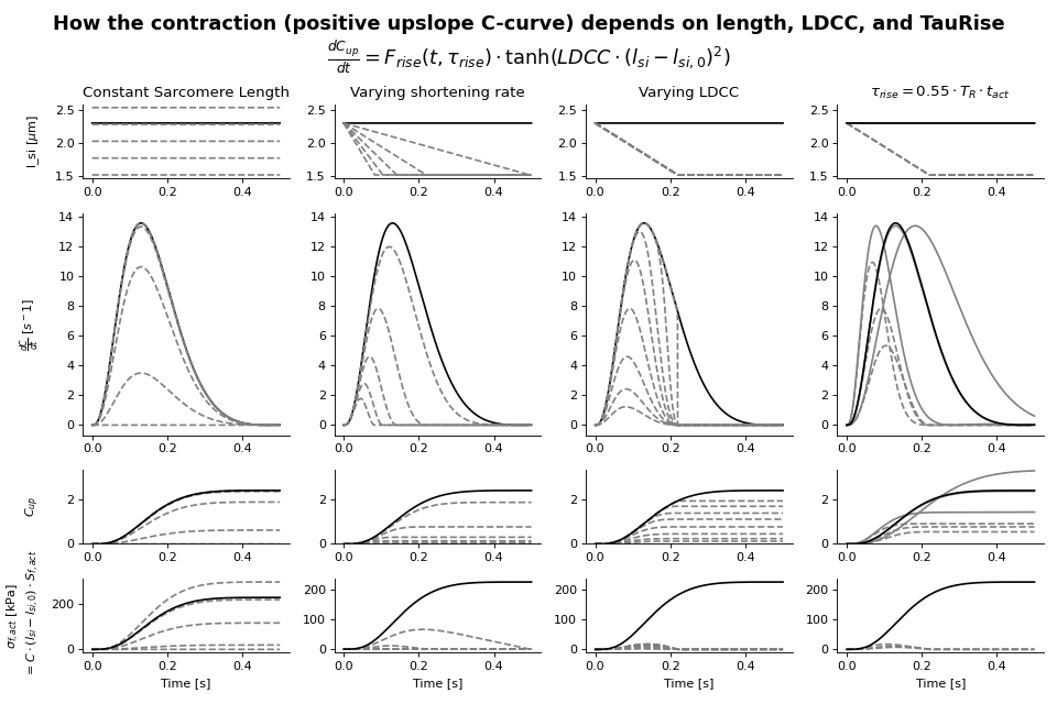
Active behavior

The active stress depends also on time through a contractility parameter \(C\). Contractility is a phenomenological quantity representing the density of cross-bridges formed in the sarcomere. There is a resting value of contractility, which may be non-zero. This can represent residual cross-bridge formation during diastole. Contractility increases when the tissue is activated. Activation is smooth and has a rise and decay phase with different time constants. The rate of change of contractility increases with sarcomere length (Kentish et al.[10]). Active stress increases with contractility, contractile element length and series elastic element length. Based on these assumptions, the contractility curve \(C\) is implemented as a state-variable and given by

(8)\[ \frac{dC}{dt} = \frac{1}{\tau_{rise}} C_L(l_{si}) \cdot f_{rise}(t) - \frac{1}{\tau_{decay}} C \cdot f_{decay}(X)\]

with

(9)\[ \begin{align}\begin{aligned} \tau_{rise}=0.55 \cdot T_r \cdot t_{duration}\\ \tau_{decay}=0.33 \cdot T_d \cdot t_{duration}\end{aligned}\end{align} \]

This function uses the function \(f_{rise}\) to modulate the rise of the contractility and \(f_{decay}\) to modulate the decay of contractility.

The first is given by:

(10)\[ f_{rise}(x_{rise}(t))=0.02x_{rise}^3 \cdot (8-x_{rise})^2 \cdot e^{-x_{rise}}\]

(11)\[ x_{rise}(t)=\min(8,\max(0,\frac{t-t_{act}}{\tau_{rise}}))\]

Crossbridge formation function \(C_L (l_{si})\)

(12)\[ C_L (l_{si} )=\tanh\left(LDCC \cdot (l_{si}-l_{si,0})^2 \right)\]

Decay function \(g(X)\)

(13)\[ f_{decay}(x_{decay}(t))=0.5+0.5 \cdot \sin\left(\text{sign}(x_{decay}) \min(\pi/2,\left|x_{decay}\right|) \right)\]

(14)\[ x_{decay}(t)=(t-t_{act}-t_{duration})/\tau_{decay}\]

From the contractility curve, the total active stress is calculated using

(15)\[ \sigma_{act}=S_{f,act} \cdot C \cdot 1.51 (\frac{l_{si}}{l_{si,0}} - 1)\cdot l_{se}/l_{se,iso}\]

(Source code, png, hires.png, pdf)

Passive behavior

(16)\[ \sigma_{ecm} = S_{f,pas} \cdot ((\frac{l_s}{l_{s,0pas}})^{k_1} - 1)\]

(17)\[ \sigma_{tit} = 0.01 \cdot S_{f,act} \cdot ((\frac{l_s}{l_{s,0pas}})^{2 \cdot l_{s,ref} / d l_{s,pas}} - 1)\]

(18)\[ \sigma_{pas} = \sigma_{ecm} + \sigma_{tit}\]

(Source code, png, hires.png, pdf)

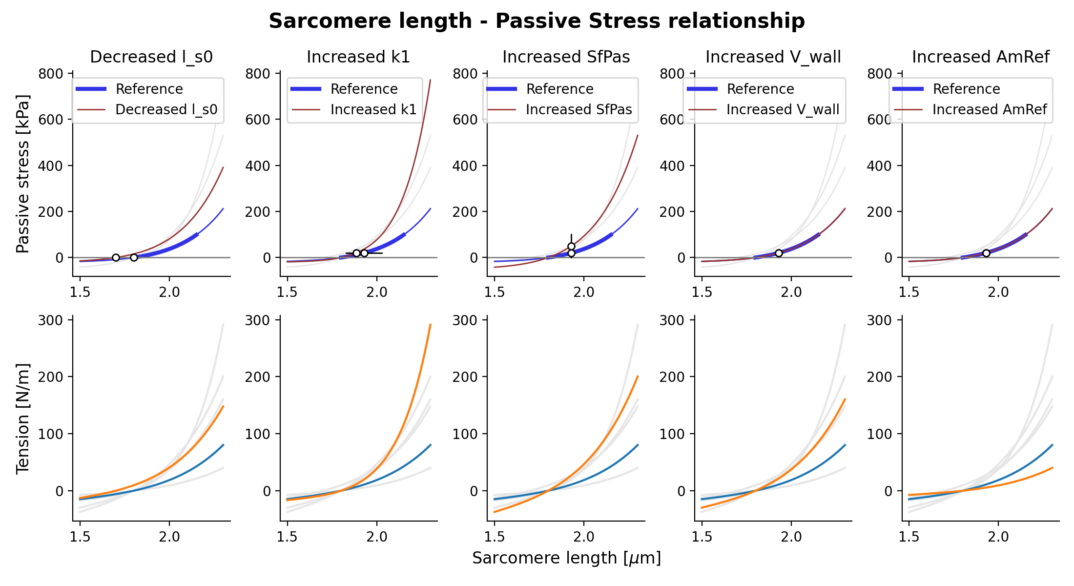
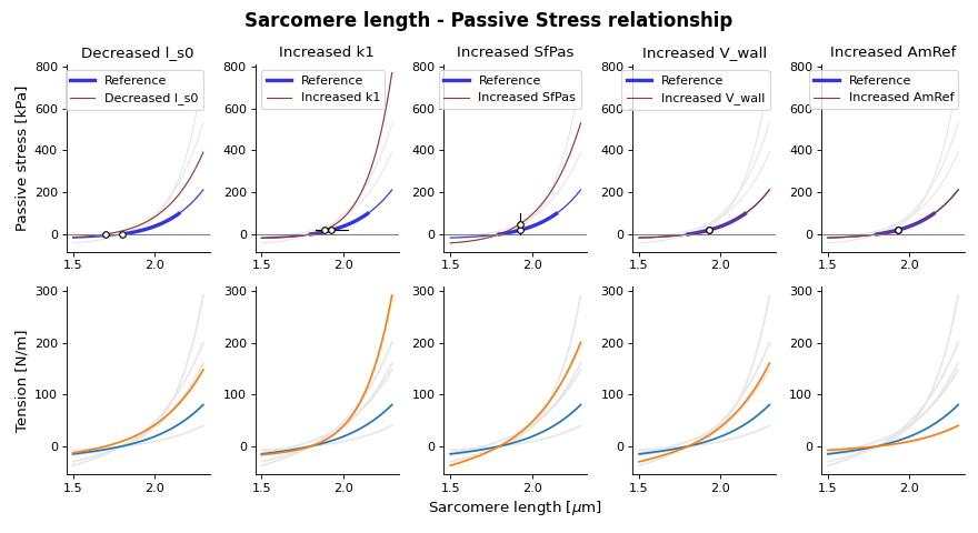
Fig. 10 Passive stress-strain relation as function of sarcomere length

(Source code, png, hires.png, pdf)

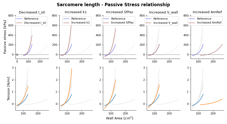
Fig. 12 Passive stress-strain relation as function of wall area

Assumptions

Not Included in this Version of the Model:

• Force-frequency relationship (force of contraction increases with heart rate).

• Electrophysiology model, only imposed activation times.

• Biophysics / energetics of calcium transient, cross-bridge formation, etc - currently, this is modelled phenomenologically and availability of ATP is assumed to be infinite.

• Sympathetic / para-sympathetic stimulation of cardiomyocytes.

References

[1]

John Walmsley, Theo Arts, Nicolas Derval, Pierre Bordachar, Hubert Cochet, Sylvain Ploux, Frits W. Prinzen, Tammo Delhaas, and Joost Lumens. Fast simulation of mechanical heterogeneity in the electrically asynchronous heart using the multipatch module. PLOS Computational Biology, 11(7):1–23, 07 2015. URL: https://doi.org/10.1371/journal.pcbi.1004284, doi:10.1371/journal.pcbi.1004284.

[2]

Daniel D Streeter Jr, Henry M Spotnitz, Dali P Patel, John Ross Jr, and Edmund H Sonnenblick. Fiber orientation in the canine left ventricle during diastole and systole. Circulation research, 24(3):339–347, 1969.

[3]

SY Ho and D Sanchez-Quintana. The importance of atrial structure and fibers. Clinical Anatomy: The Official Journal of the American Association of Clinical Anatomists and the British Association of Clinical Anatomists, 22(1):52–63, 2009.

[4]

Theo Arts, Tammo Delhaas, Peter Bovendeerd, Xander Verbeek, and Frits W Prinzen. Adaptation to mechanical load determines shape and properties of heart and circulation: the circadapt model. American Journal of Physiology-Heart and Circulatory Physiology, 288(4):H1943–H1954, 2005.

[5] (1,2,3,4)

Joost Lumens, Tammo Delhaas, Borut Kirn, and Theo Arts. Three-wall segment (triseg) model describing mechanics and hemodynamics of ventricular interaction. Annals of biomedical engineering, 37:2234–2255, 2009.

[6]

Joost Lumens, Sylvain Ploux, Marc Strik, John Gorcsan, Hubert Cochet, Nicolas Derval, Maria Strom, Charu Ramanathan, Philippe Ritter, Michel Haïssaguerre, and others. Comparative electromechanical and hemodynamic effects of left ventricular and biventricular pacing in dyssynchronous heart failure: electrical resynchronization versus left–right ventricular interaction. Journal of the American College of Cardiology, 62(25):2395–2403, 2013.

[7]

James A Goldstein, James S Tweddell, Benico Barzilai, Yoko Yagi, Allan S Jaffe, and James L Cox. Hemodynamic effects of atrial interaction. Coronary Artery Disease, 4(6):545–553, 1993.

[8]

Mark Henein, Yat-Yin Lam, Anders Waldenstöm, and Michael Y Henein. Atrial interaction in the form of ‘cross talk’in patients with ventricular outflow tract obstruction. International journal of cardiology, 147(3):388–392, 2011.

[9]

Yuan-Cheng Fung. Mathematical representation of the mechanical properties of the heart muscle. Journal of biomechanics, 3(4):381–404, 1970.

[10]

Jonathan C Kentish, HE Ter Keurs, Lucio Ricciardi, JJ Bucx, and MI Noble. Comparison between the sarcomere length-force relations of intact and skinned trabeculae from rat right ventricle. influence of calcium concentrations on these relations. Circulation research, 58(6):755–768, 1986.

circadapt.components.patch.Patch2022(model)

Patch2022 is based on Patch in Walmsley 2015.