Tags: Valve2022

Verification of Valve2022

In order to verify the Valve2022, a benchmark model is designed in which the Valve2022 has a prescribed proximal and distal pressure and area.

Code Verification of the State Variable \(q\)

The Valve2022 module solves the differential equation:

\[\frac{dq}{dt} = \frac{1}{L_{total}} \cdot \Bigg({\Delta}p_{bernoulli} - {\Delta}p\Bigg)\]

This benchmark setup places the Valve2022 module in a setup with prescribed constant proximal and distal pressures. The proximal pressure is a stepfunction, for which the pressure is \(p=2000Pa\) for \(0.1<t<0.4\) and \(p=0Pa\) elswhere. The distal pressure is constant at \(p=1000Pa\). This results in a \(\Delta p = \pm 1000Pa\).

This benchmark problem has 3 phases. Phase 1 has a negative pressure drop with a positive decreasing flow. Phase 2 has a negative pressure drop with a negative stabalizing flow. Phase 3 has a positive pressure drop with a positive increasing to stabalizing flow. After phase 3, phase 1 is repeated.

Two different valve states occur in these phases, namely open and closed valve. This results into 3 different analytical solutions for each of the phases.

To analytically solve the equation, we rewrite the equation into

\[\frac{dq}{dt} = \frac{1}{L_{total}} \cdot \Bigg(\alpha q |q| - {\Delta}p\Bigg)\]

In this equation, \(L_{total}\) is given by

\[L_{total} = \rho_b \cdot \Bigg( \alpha_{valve} \cdot \frac{l}{A} + \frac{\alpha_{prox}}{\sqrt{A_{prox}}} + \frac{\alpha_{dist}}{\sqrt{A_{dist}}} \Bigg)\]

in which \(A_{eff}=A_{open}\) if \(\Delta p<0\) and \(A_{eff}=A_{leak}\) if \(\Delta p>=0\). Furthermore, \(\alpha\) is given by

\[\begin{split}\begin{matrix} \alpha = \alpha_{open} = \frac{1}{2} \rho \big( \frac{1}{A_{prox}^2} - \frac{1}{A_{eff}^2} \big) & \text{if} q>0 \text{or} \Delta p < 0 \\ \alpha = \alpha_{leak} = \frac{1}{2} \rho \big( \frac{1}{A_{eff}^2} - \frac{1}{A_{dist}^2} \big) & \text{else} \end{matrix}\end{split}\]

As a result of the \(|q|\), there are two analytical solutions. One for positive flow and one for negative flow. Additionally, the constant \(\alpha\) changes when

Phase 1: Positive pressuredrop with positive decreasing flow

\[q(t) = -\sqrt{\frac{\Delta p}{\alpha_{open}}} \tan\left(\frac{\sqrt{\alpha_{open} \cdot \Delta p}}{L}t + c_1 \sqrt{\alpha_{open} \cdot \Delta p}\right)\]

with \(c_1\) such that \(q(0) = q_0\). Notably in this analytical solution is that if \(\Delta p\) is negative, \(\alpha\) is also negative. Consequently, must be \(A_{open} < A_{prox}\). The limit of these solution goes to \(q=-\infty\), however, it will go to phase 2 when the sign of \(q\) changes negative.

Phase 2: Positive pressuredrop with negative flow

\[q(t) = -\sqrt{\frac{\Delta p}{\alpha_{leak}}} \tanh\left(\frac{\sqrt{\alpha_{leak} \Delta p}}{L} t + c_2 \sqrt{\alpha_{leak} \Delta p}\right)\]

with \(c_2\) such that \(q(t_2) = 0\). This phase is stable, with an asympote at \(q=-\sqrt{-\frac{\Delta p}{\alpha_{leak}}}\).

Phase 3: Negative pressuredrop

\[q(t) = \sqrt{\frac{\Delta p}{\alpha_{open}}} \tanh\left(-\frac{\sqrt{- \alpha_{open} \Delta p}}{L} t + c_3 \sqrt{\alpha_{open} \Delta p}\right)\]

with \(c_3\) such that \(q(t_3) = 0\). This phase is stable, with an asympote at \(q=\sqrt{\frac{\Delta p}{\alpha_{open}}}\)

Verification

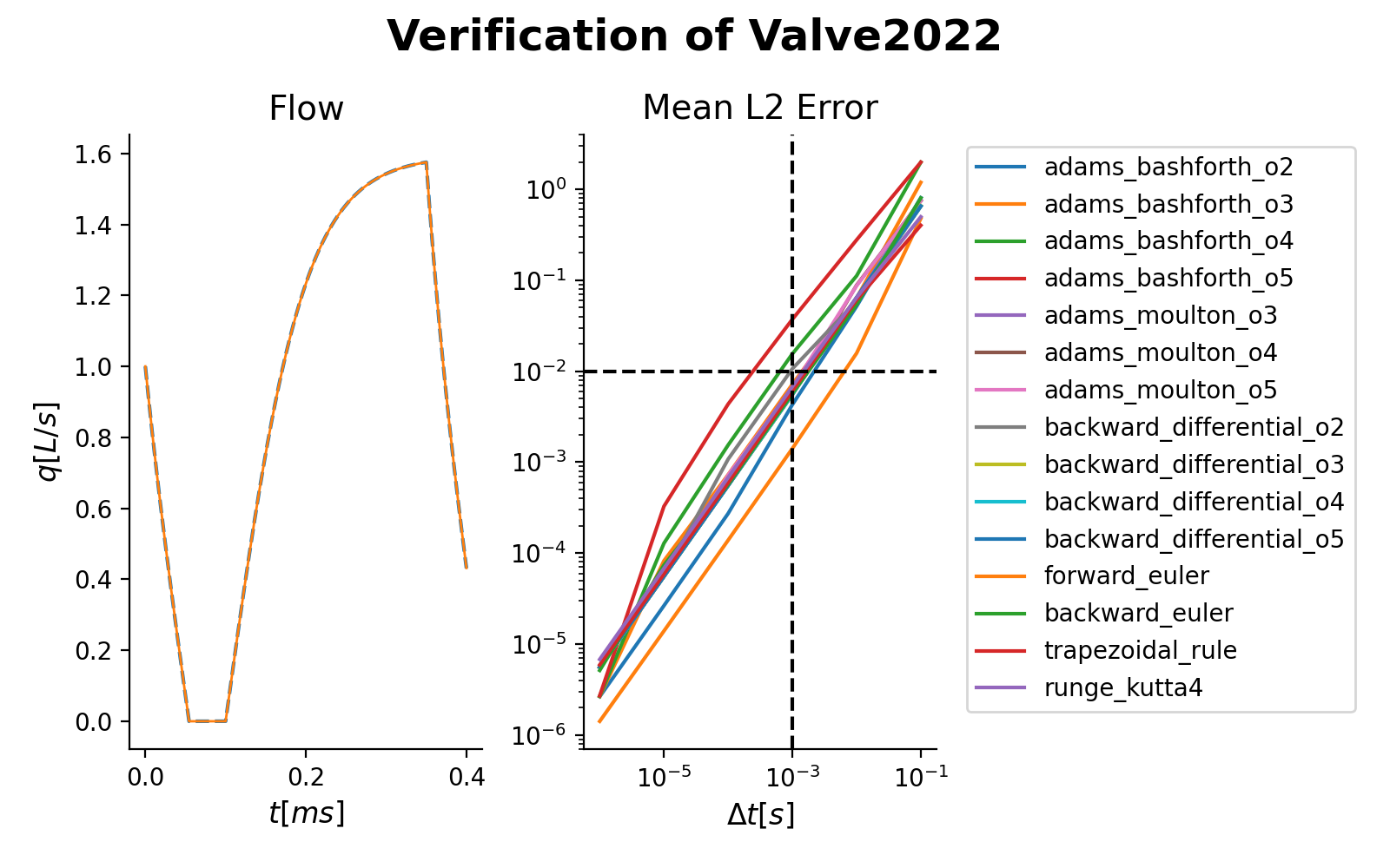
(Source code, png, hires.png, pdf)

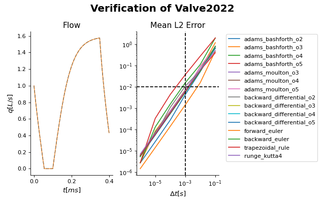
Fig. 18 Verification of the Valve2022 module. Left: True solution of the flow pattern (solid) with the forward euler solution at \(\Delta t = 5e-3ms\). Note the overshoot when the sign of the flow turns negative, which is more pronound at larger timesteps. Right: Mean L2 error, defined as \(\sum_t \frac{\Delta t}{t_{cycle}} \frac{q_{true}(t) - q_{model}(t)}{\overline{q_{true}}}\), as a function of the timestep \(\Delta t\) for different numerical solvers. At \(\Delta t = 1ms\), all numerical solvers have mean L2 \(<1e-2\) except for the 4th and 5th order adams bashforth method.