Valve2022
Module summary
Module to simulate valvular flow.
This model simulates flow \(q\) based on the pressure gradient between the proximal and distal node \(\Delta p\) by solving the ordinary differential equation:
Parameters
- adaptation_Aopen_fac [-]: double
Factor used in adaptation to determine Aopen based on vessel flow.
- A_open [m2]: float
Opening area
- A_leak [m2]: float
Leaking valve area
- l [m]: float
Length of valve
- rho_b [kg/m3]: float
Blood density
- papillary_muscles [-]: bool
If true, papilary muscle implementation is activated
- soft_closure [-]: bool
If true, a soft closure is activated
Signals
- q [m3/s]: float
Flow through the valve
- dq_dt [m3/s2]: float
Time derivative of the flow q
Physiological background
In a normal adult, the heart has four chambers, i.e., the left (LA) and right atrium (RA) and the left (LV) and right ventricle (RV). The heart valves are the orifices which connect atrium to ventricle and ventricle to artery, or also known as atrioventricular and ventriculo-arterial valves, respectively. Besides the latter valves, the atrial myocardial walls contain other (permanently open) orifices connecting the systemic veins with the RA and the pulmonary veins with the LA.
Atrioventricular (AV) and ventriculo-arterial valves
There are two atrioventricular valves, i.e., the mitral valve separating the LA from the LV, and the tricuspid valve, separating the RA from the RV. The two ventriculo-arterial valves are the aortic valve, separating the LV from the aorta, and the pulmonary valve, separating the RV from the pulmonary artery.
Opening of the valves is driven by a transvalvular pressure drop. During diastole, the atrioventricular valves are open, allowing the ventricles to be filled with blood. When the pressure in the ventricles exceeds that in the atria, these valves will start to close. This closure will occur gradually due to inertia of the accelerated blood volume. Similarly, when ventricular pressure exceeds that in the distal arteries, the ventriculo-arterial valves open and blood leaves the ventricles, reducing the volumes of the ventricles. The atria are in open connection with the venous circulation, allowing continuous flow into the atria.
Atrioventricular regurgitation and prolapse due to high pressures in the ventricles during systole are prevented by papillary muscle contraction. The LV papillary muscles attach the two cusps of the mitral valve to the anterior and posterior LV free wall. The RV papillary muscles attach the three cusps of the tricuspid valve to the anterior and posterior RV free wall and the septum. Normally, the papillary muscles are activated simultaneously with the ventricular myocardium and maintain tension throughout the entire systolic phase, thereby preventing backflow into the ventricle.
Valvular stenosis is an abnormal (disease) condition, in which the tissues forming the valve leaflets have become stiffer and thereby reduce the normal valve opening area. As a result, forward blood flow through the valve is restricted so that the proximal cardiac chamber needs to work harder to eject the same amount of blood. Valvular insufficiency is an abnormal (disease) condition, in which the valve leaflets do not close properly, so that blood can flow backward across the valve.
The Valve2022 Module
The valve module can be used to model any narrow orifice in the circulation where passing blood flow causes a pressure drop related to inertia and Bernoulli effect in both physiology and pathophysiology. The valve module can connect any pair of Node & Cavity objects in pure form or modeled as e.g. Chamber2022, TriSeg2022, or Tube0D. Examples of these combinations are chamber-to-tube (aortic and pulmonary VA valves), tube-to-chamber (veno-atrial inlets), chamber-to-chamber (mitral and tricuspid valves, ASD and VSD), and tube-to-tube (systemic-to-pulmonary artery shunt).
The state variable in this module is blood flow q through the valve. The module adds an ordinary differential equation \(dq/dt = f(q, \Delta p)\) to the system of equations solved in CircAdapt.
Physical background
The Navier-Stokes equation describes the relation between pressure p and flow velocity v in a flow field of an incompressible fluid:
where symbols \(\rho_b\) and \(\eta\) refer to blood density and viscosity, respectively. In a cylindrical tube, assuming laminar flow and dominance of flow velocity \(v_z\) in the axial z-direction, Equation 1 is simplified to:
Integration along a stream line, neglecting viscosity and the effect of gravity over the short distance within the valve, for the pressure difference \(\Delta p\) over a trajectory it follows:
The direction of the flow is from proximal to distal. The pressure drop is defined as
For steady state flow, proximal to the valve orifice streamlines are converging (Fig. 6) in a practically laminar fashion, allowing application of Equation 3. However, distal to the orifice, streamlines diverge, generally resulting in vortices and turbulence with loss of energy. In the valve module we assumed that no pressure is regained by deceleration of the blood distal to the orifice. As a result, flow through the valve is a result of the transvalvular pressure (\(\Delta p\)), the Bernoulli pressure gradient between the proximal node and the flow in the valve (\(\Delta p_{bernoulli} = \frac{1}{2}\rho v^2\)), and inertia due to acceleration in time (\(dv_z/dt\)).

Fig. 11 Principle of Bernoulli’s equation. With converging stream lines, accelerating flow remains mostly laminar, allowing application of Bernoulli’s equation. With decelerating flow, often turbulence occurs, causing loss of kinetic energy.

Fig. 12 Schematic representation of a valve. Symbols p, q, A and l represent pressure, flow, crosssectional area and section length, respectively. Subscripts prox, valve and dist refer to proximal, valve orifice and distal, respectively.
Model Description
The valve in the CircAdapt model is based on Equation 3. For proper incorporation in the model velocity \(v_z\) is not directly available. Instead we used the state variable flow \(q\). The following assumptions and simplifications were applied:
Blood is an incompressible, i.e., Newtonian fluid
The valve is assumed to be a cylindrical tube with laminar flow and dominance of \(v_z\)
The effect of gravity and viscosity is neglected
There is no flow gradient perpendicular to streamlines
A representative value for velocity is obtained by flow q divided by effective area \(A\)
At the inlet side all pressure-flow energy is converted to kinetic energy
At the outlet side, pressure is not regained even though velocity is decreasing, implying loss of energy to be attributed to turbulence and viscous losses.
Distal to the valve orifice, kinetic energy \(E_{kin}\) is lost to the level of exit velocity
Inertia L is estimated using the equation \(E_{kin} = \frac{1}{2} L q^2\)
Given a steady state flow q, thereby neglecting the time-dependent term, the pressure drop \(\Delta p\) over the valve, as sketched in Fig. 12, is determined by the Bernoulli equation, as shown in Equation 3 without the time-dependent term:
The first term refers to the proximal side of the valve, where laminar flow without energy loss is assumed to hold. The second term considers regaining of pressure in a divergent flow field. We assumed there is no regain, implying \(c_{dist}\). If some pressure is regained, i.e., \(c_{dist}>0\), we may assume an effective valve cross-section \(A_{eff}\) in stead of \(A_{valve}\). Note that \(\Delta p\) is negative, since in general it holds \(A_{eff}<A_{prox}\).
To express the effect of inertia L, we now consider flow dynamics. The total kinetic energy \(E_{kin}\) equals the volume integral of the Bernoulli pressure over the whole valve and the proximal and distal volumes. Assuming that flow is the same within each section, and velocity equals flow q divided by area \(A\), the total kinetic energy equals
Using \(E_{kin} = \frac{1}{2} L q^2\),
In this equation all length and area parameters are condensed to the ratio of an effective length \(l_{eff}\), and an effective area \(A_{eff}\) as determined in Equation 7 for steady state flow.
Flow velocity is known not to be uniform. E.g., flow entering an orifice is contracting towards the center of the orifice, making the effective orifice \(A_{eff}\) to be smaller than the physical orifice size. Furthermore, inertia \(L\) is known to depend on the distribution of flow velocity within the valve region. By choosing an appropriate value for \(l_{eff}\) the effect of inertia can be approximated quite well, while the number of valve parameters remains limited. For an orifice with negligible length, the effective length \(l_{eff}\) is quite well approximated by the diameter of the orifice. Integrating all above into Equation 3 renders
Rewriting of Equation 8 results in the ordinary differential equation
The characteristics of a valve depend typically on the flow direction. If flow reverses, in we should interchange proximal and distal. For regular valves, forward and backward flow behavior is very different. With forward flow \(A_{eff}\) is much larger than with backflow. In the implementation, \(A_{eff}\) is always kept positive to avoid zero-division. The value of \(l_{eff}\) is less critical for change of flow direction, and is therefore kept constant. The CircAdapt program requires the time derivative of flow \(dq/dt\) to be written explicitely as a function of the pressure drop \(p_{drop}\), being the negative of \(\Delta p\).
Numerical implementation
In the numerical implementation, this equation is rewritten to
In which \({\Delta}t / \tau\) is added for numerical stability at low flows and \(L_{total}\) is given by
In the publication by Walmsley et al. Plos 2015, inertia factors were \(\alpha_{valve}=1.5\), \(\alpha_{prox}=0.75\), \(\alpha_{dist}=0.75\) In a the model VC04, inertia factors were \(\alpha_{valve}=1.33\) approximating a parabolic flow pattern, and \(\alpha_{prox}=\alpha_{dist}=0\) ignoring the effects of the proximal and distal node.
The pressure drop \(\Delta p\) is the difference between distal and proximal pressure. The pressure drop \(\Delta p_{bernoulli}\) with \(q>0\) is given by
The pressuredrop \(\Delta p_{bernoulli}\) with \(q<0\) is given by
The verification of this module can be found here
Valve opening and closure
Obviously, a regular valve closes if flow q reverses. However, if the pressure drop \(p_{drop}\) acts in the reverse direction, the valve remains open, as long as flow is forward (i.e., inertia dominated). In the aortic valve, such situation occurs in the late phase of systole. Then, aortic flow decelerates while aortic pressure exceeds left ventricular pressure. Valve closure occurs if flow changes sign.
In open condition, the area of the valve (\(A_{eff}\)) is set to \(A_{open}\). When the valve in the model is closed, \(A_{eff}\) is set to near-zero (\(A_{leak}\)) to prevent zero-division. As a result, there is a very high reversed modelled flow velocity when a valve is closed. If a positive pressure gradient is regained, the leakage flow needs time to decelerate due to the inertia of the narrow flow channel according to the model.
In the real situation, because of the very flexible valve leaflet material the aortic valve opens immediately at the moment the pressure drop becomes positive. To take this into account, the following criteria for valve opening and closure were used
if \(q>0 \lor {\Delta}p<0\) → open
if \(q<0 \land {\Delta}p>0\) → closed
With open valve, orifice area \(A_{eff}\) is set to \(A_{open}\) and with the closed valve to \(A_{leak}\).
Papillary Muscle Function
The Valve2022 module has optional papillary muscle function. If ‘papillary_muscles==False’, the parameter ‘A_leak’ is used to describe leaking area during back flow. If ‘papillary_muscles==True’, effective Aleak is described by:
with \(T_m\) the tension on the midwall of the Wall2022 to which the papillary muscles are attached, \(\frac{dA_m}{dT_m}\) the area-tension derivative and \(A_{m,0}\) the linearized stress-free area.
Soft Closure
In reality, the valve does not close immediately. This behavior is simulated using the soft closure option, which not only replicates the real-world dynamics more accurately but also enhances numerical stability by reducing the stiffness of the ordinary differential equation (ODE) at the point of closure. If activated, the valve area \(A_{valve}\) is changed in case there is a positive pressure gradient and positive flow:
with forward energy \(E_{forward}\) and reference energy \(E_{ref}\) defined as
As a result, \(A_{valve}=A_{open}\) with a negative pressure gradient, \(A_{valve}=A_{leak}\) with a positive pressure gradient and negative flow, and \(A_{leak}<A_{valve}<A_{open}\) while closing (positive flow with positive pressure gradient).
Add Valve2022 to custom model configuration
When building your own model, you can add a Valve2022 object to your model using:
import circadapt
model = circadapt.CircAdapt('forward_euler')

...
# Create node N and M. Could be any Node or Cavity type.
model.add_component('Tube0D', 'N')
model.add_component('Tube0D', 'M')
...
# Add a valve between N and M
model.add_component('Valve2022', 'N2M')
model.set_component('N2M.prox', 'N')
model.set_component('N2M.dist', 'M')
...
This code will add a valve between two Tube0D objects named N and M. The valve module does not behave properly when:
Proximal or distal node are not set.
Proximal or distal node have wave impedance of zero.
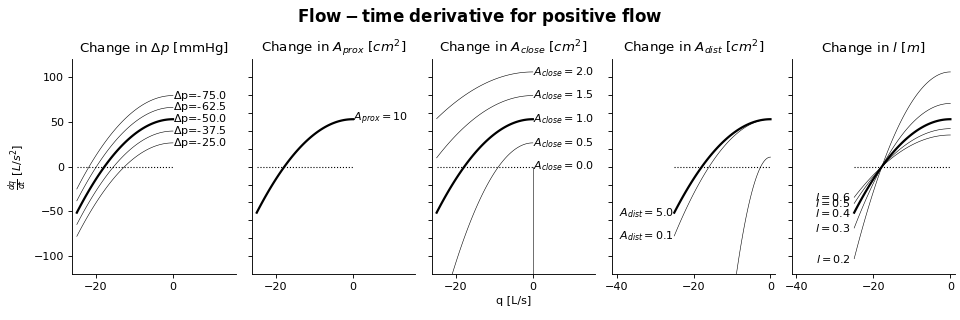
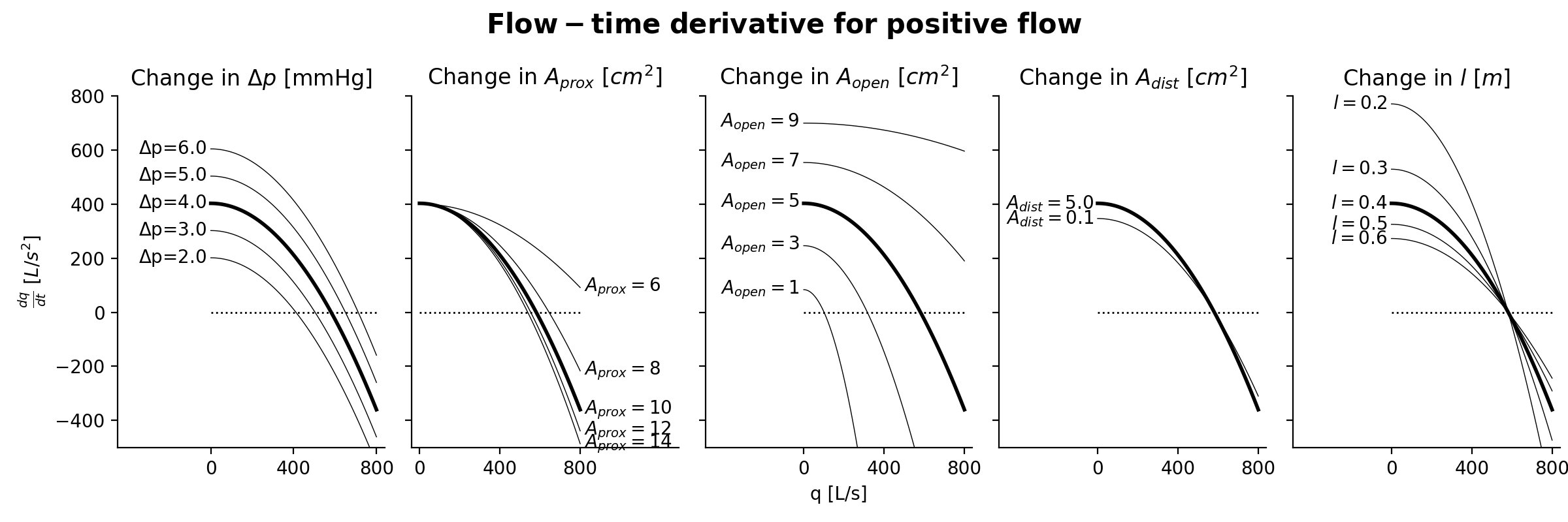
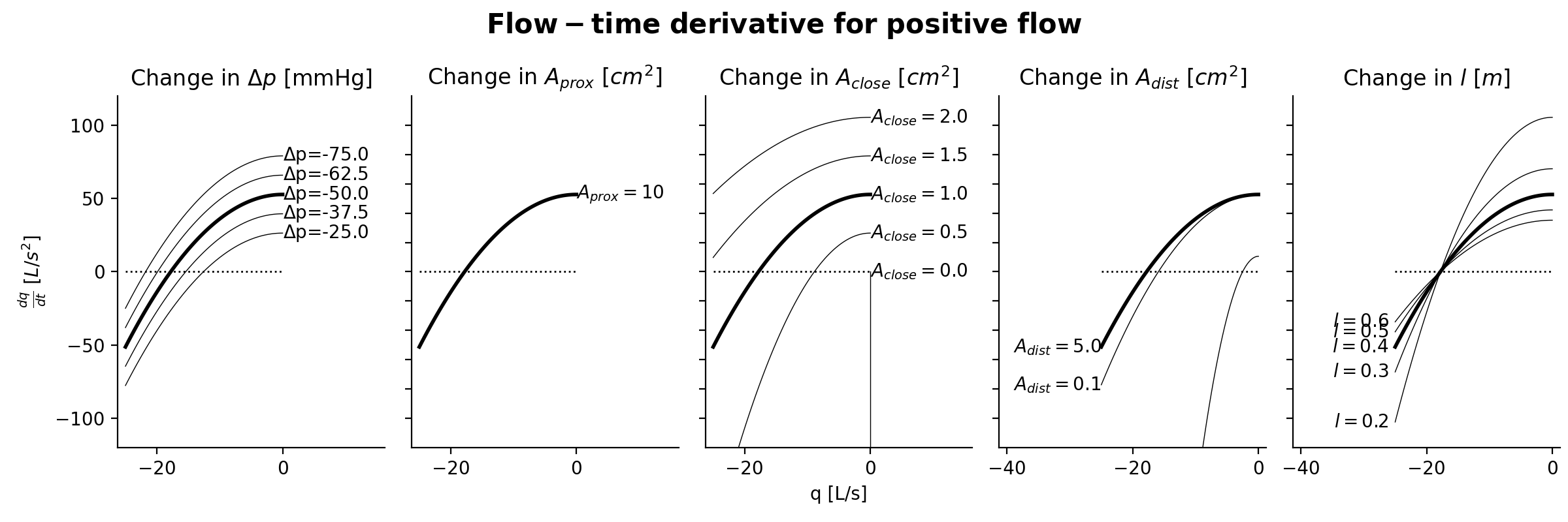
Sensitivity Analysis
More information on how to read the Sensitivity Analysis here.
(Source code, png, hires.png, pdf)

(Source code, png, hires.png, pdf)