VanOsta2022 Regional Myocardial (Dys)function

The multipatch implementation of the wall module allows for simulationg regional wall mechanics. To initiate this, the wall can be split in multiple patches using the lines:

model['Wall']['n_patch'][2:4] = [12, 6]

In this example, we apply a small heterogeneity in activation delay.

model['Patch']['dt'][2:14] = np.linspace(0, 0.02, 12)
model['Patch']['dt'][14:20] = np.linspace(0.01, 0.05, 6)

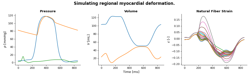
Running this simulation results in the following pressures, volumes, and regional fiber strain.

(Source code, png, hires.png, pdf)

The full code to generate this plot is shown below.

"""
Tutorial CircAdapt VanOsta2022.

March 2023, by Nick van Osta

This tutorial demonstrates how to model regional mechanics, how to change
regional parameters and how to obtain and plot regional
"""

import numpy as np
import matplotlib.pyplot as plt
import circadapt
from circadapt.model import VanOsta2023

# %% 1. load model
model = VanOsta2023()

# Split the LV in 12 and SV in 6 segments
model['Wall']['n_patch'][2:4] = [12, 6]

# Set activation delay
model['Patch']['dt'][2:14] = np.linspace(0, 0.02, 12)
model['Patch']['dt'][14:20] = np.linspace(0.01, 0.05, 6)

# Run beats
model.run(stable=True)

# Plot data
fig = plt.figure(2, figsize=(13, 4))
ax1 = fig.add_subplot(1, 3, 1)
ax2 = fig.add_subplot(1, 3, 2)
ax3 = fig.add_subplot(1, 3, 3)

# Plot pressure
ax1.plot(model['Solver']['t']*1e3,
         model['Cavity']['p'][:, ['cLv', 'SyArt', 'La']]*7.5e-3,
         )

# Plot Volume
ax2.plot(model['Solver']['t']*1e3,
         model['Cavity']['V'][:, ['cLv', 'La']]*1e6,
         )

# Plot natural fiber strain
ax3.plot(model['Solver']['t']*1e3,
         model['Patch']['Ef'][:, 2:20],
         )

# plot design, add labels
for ax in [ax1, ax2, ax3]:
    ax.spines[['right', 'top']].set_visible(False)
ax2.set_xlabel('Time [ms]', fontsize=12)

ax1.set_ylabel('$p$ [mmHg]', fontsize=12)
ax2.set_ylabel('$V$ [mL]', fontsize=12)
ax3.set_ylabel('$\epsilon$ [-]', fontsize=12)

ax1.set_title('Pressure',
             fontsize=12, fontweight='bold')
ax2.set_title('Volume',
             fontsize=12, fontweight='bold')
ax3.set_title('Natural Fiber Strain',
             fontsize=12, fontweight='bold')

fig.suptitle('Simulating regional myocardial deformation. ',
             fontsize=15, fontweight='bold')

plt.tight_layout()
plt.draw()