VanOsta2022 Physiology

Tags: Bag

(Source code)

(png, hires.png, pdf)

(png, hires.png, pdf)

python

"""
Tutorial CircAdapt VanOsta2022.

November 2022, by Nick van Osta

The goal of this tutorial is to understand the CircAdapt framework and to use
the VanOsta2022 model. This tutorial assumes little to no knowledge about
python. Therefore, basic python conventions and syntax will be discussed.
This tutorial assumes the installation is followed as described on the wiki
(https://wiki.circadapt.org/index.php?title=Circadapt_in_Python). This uses
Python >3.9 installed with anaconda and editted in Spyder. Other ways are
possible, but might not be in line with this tutorial.

Content
-------
    1. Basics of python
    2. Load the model
    3. Plot global hemodynamics
    4. Change parameters
    5. Multipatch and local dynamics
    6. Save and Load
"""

# %% 1. Basics of python
print('1. Basics of python')

# Always start the document with importing modules.
# Numpy is used for mathematics, Matplotlib for plots. These are conventionally
# imported as np and plt.
import numpy as np
import matplotlib.pyplot as plt

# Only import the class we need in this tutorial.
from circadapt import VanOsta2022
# CA = VanOsta2022()

# alternatively, you can import the whole package, but it changes the way you
# make the object.
# import circadapt
# CA = circadapt.VanOsta2022()

# Parameters types are automaticaly set or changed by the interpreter, but it
# is good to create an integer when you need an integer and float when needed.
i = 1                 # integer
f = 1.                # float
b = True              # bool
l = [1, 2, 3]         # list
d = {'a': 1, 'b': 2}  # dictionary

# get data from the list and dictionary
first_item_of_list = l[0]
item_from_dictionary = d['a']

# the use of numpy is advised for more complex use and for calculation
numpy_array = np.array(l)
print('Find if array is 2: ', (numpy_array == 2))
print('Multiply array with 2: ', (numpy_array * 2))

# In spyder, you can place bullits. While debugging, ipython will stop at these
# bullits. You can also press f9 to run a single line or selection and press
# crtl+<enter> to run a block seperated by # %%

# %% 2. load model
print('\n 2. Load model. ')
# Load predefined model with predefined parameterization
# More information on this model can be found here:
# https://wiki.circadapt.org/index.php?title=VanOsta2022
CA = VanOsta2022()

# CircAdapt tries to follow the syntax of python and numpy as much as possible.
# The object can be handled as a dictionary. Content can be printed in the
# console, and printed on request in the ipython console.
print('The result of printing the object gives information about the '
      'components: ')
print(CA)

# components can also be retrieved as a list of strings
components = CA.components
print('Components of this model: ', components, '\n')

# Similar to the object itself, components can be printed
print('Patches in this model: ')
print(CA['Patch2022'])

# Each component points to multiple c++ objects of that component type. The
# objects can also be obtained using
objects = CA['Patch2022'].objects
parameters = CA['Patch2022'].parameters
signals = CA['Patch2022'].signals

# Signals are not stored, so they are only available after running a beat.
# Therefore the model should run. You can either run a number of beats, or run
# until the model is hemodynamically stable.
CA.run(5)
CA.run(run_stable=True)

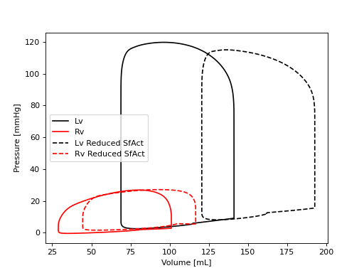
# %% 3. Plot global hemodynamics
# Here is an example code to plot the PV loop
# First we open a figure. Assigning this figure to a variable is optional, but
# is useful for design purposes.
fig = plt.figure(1)

# get volume and pressure of LV
Vlv = CA['Cavity']['V'][:, 6]*1e6
plv = CA['Cavity']['p'][:, 6]*7.5e-3

# get volume and pressure of RV
Vrv = CA['Cavity']['V'][:, 7]*1e6
prv = CA['Cavity']['p'][:, 7]*7.5e-3

# You can also use location names to get/set signals and parameters
# For this, use only the last part of the full object name, e.g. cLv for
# Model.Peri.TriSeg.cLv. You can get one signal or multiple signals
Vlv = CA['Cavity']['V'][:, 'cLv']*1e6
Vrv = CA['Cavity']['V'][:, 'cRv']*1e6
pressure = CA['Cavity']['p'][:, ['cLv', 'cRv']]*7.5e-3

# you can split the two pressure signals into two parameters using the
# following line. First transpose the pressure such that the first axis sets
# the signals
plv, prv = pressure.T

# Now we plot the two lines.
line1 = plt.plot(Vlv, plv, c='k', label='Lv')
line2 = plt.plot(Vrv, prv, c='r', label='Rv')
plt.ylabel('Pressure [mmHg]')
plt.xlabel('Volume [mL]')
plt.legend()

# %% 4. Change parameters
# Now reduce the contractility of all 3 ventricular walls, run the simulation,
# and plot the data
CA['Patch2022']['SfAct'][2:] = 60e3
CA.run(run_stable=True)
plt.plot(CA['Cavity']['V'][:, 6]*1e6, CA['Cavity']['p'][:, 6]*7.5e-3, 'k--', label='Lv Reduced SfAct')
plt.plot(CA['Cavity']['V'][:, 7]*1e6, CA['Cavity']['p'][:, 7]*7.5e-3, 'r--', label='Rv Reduced SfAct')
plt.legend()


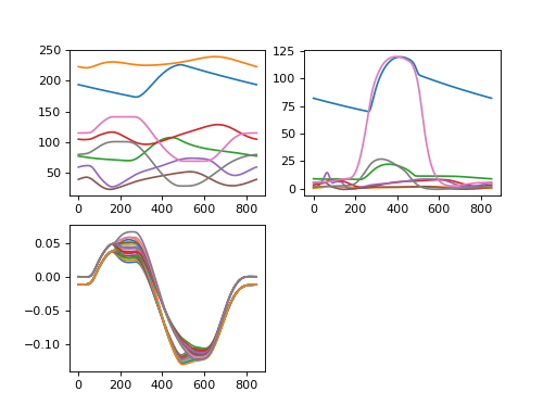
# %% 5. Multipatch and local dynamics
# Set up a new multipatch model and set an activation delay
CA_multipatch = VanOsta2022()

# The number of patches is specified in the wall. Here, we set 12 Lv patches
# and 6 Sv patches. Then, we change the dT in these patches.
CA_multipatch['Wall2022']['n_patch'][2:4] = [12, 6]
CA_multipatch['Patch2022']['dT'][2:14] = np.linspace(0, 0.01, 12)
CA_multipatch['Patch2022']['dT'][14:20] = np.linspace(0, 0.01, 6)

# Run beats
CA_multipatch.run(run_stable=True)

# Plot data
fig = plt.figure(2)

# In the first subplot, plot all volumes
ax1 = plt.subplot(2, 2, 1)
plt.plot(CA_multipatch['Solver']['t']*1e3,
         CA_multipatch['Cavity']['V']*1e6,
         )
# in the second subplot, plot all pressures
ax1 = plt.subplot(2, 2, 2)
plt.plot(CA_multipatch['Solver']['t']*1e3,
         CA_multipatch['Cavity']['p']*7.5e-3,
         )
# in the third subplot, plot all natural fiber strains.
ax1 = plt.subplot(2, 2, 3)
plt.plot(CA_multipatch['Solver']['t']*1e3,
         CA_multipatch['Patch2022']['Ef'][:, 2:20],
         )

# %% 6. Save and Load
# Simulations can be saved and loaded using the following code.
CA_reference = VanOsta2022()

# use .npy extension in filename
CA_reference.save('reference.npy')

# ander bestand
model = VanOsta2022()
model.load('reference.npy')

# if you want to save and load a structure without writing it to a file, use
# the follow lines. Note that signals are not filled, you have to run at least
# 1 beat.
data = CA_reference.model_export()
CA_reference.model_import(data)

Detailed tutorials

• VanOsta2022 Valvulopathies
• VanOsta2022 Systemic Circulation