Preload Afterload experiment
Tutorial on how to implement the preload-afterload experiment. This tutorial discusses how to build the model, how to switch between different patch types, and how to extract and plot information from the model.
Todo
Make Preload Afterload methods figure
As all projects, we start with importing packages.
 1# sys.path.append('../../../src/')
 2
 3import circadapt
 4# Uncomment next lines if not installed
 5# circadapt.DEFAULT_PATH_TO_CIRCADAPT = "../../../core/out/build/x64-Release/CircAdaptLib.dll"
 6
 7
 8
 9# import
10from circadapt import CircAdapt
11import numpy as np
12import matplotlib.pyplot as plt
13
14import time
15
We then create an empty model. Then, we add the PreAfterloadExperiment wall object. This object is empty by default, but it needs at least 1 patch object to work. In this tutorial, we use the Patch2022 object.
1model = CircAdapt(
2    'Custom',
3    'SolverFE',
4    )
5model.add_component('PreAfterloadExperiment', 'PAE')
6model.add_component('Patch2022', 'P', 'PAE')
7
The model has to be parametized, as default parameter values do not make sense for this setup.
 1model.set('Model.tCycle', 1e-0)
 2model.set('Solver.dT', 1e-3)
 3model.set('Solver.dTexport', 1e-3)
 4
 5model['PreAfterloadExperiment']['AmRef_Afterload'] =  0.006
 6model['PreAfterloadExperiment']['T_afterload'] =  200
 7model['PreAfterloadExperiment']['n_iter'] =  5
 8model['Patch2022']['AmRef'] =  0.005
 9model['Patch2022']['VWall'] = 92.43*1e-6
10model['Patch2022']['ADO'] = 3.0
11model['Patch2022']['TR'] = 0.5
12model['Patch2022']['TD'] = 0.5
13model['Patch2022']['k1'] = 10.
14model['Patch2022']['vMax'] = 7.0
15model['Patch2022']['dT'] = 0.1
16
17model.set('Model.PAE.P.Lsi', -0.04 + 2 * np.sqrt(
18    model['PreAfterloadExperiment']['AmRef_Afterload'][0]/model['Patch2022']['AmRef'][0]))
19
Now the model setup is finished and we can run the simulation. For this setup, only 1 run is sufficient.
1t0 = time.time()
2model.run(1)
3t1 = time.time()
4print(t1-t0)
5
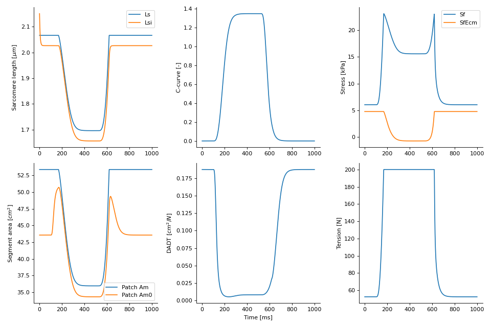
The simulation will result in the stresses and tensions shown in the plot below.
(Source code, png, hires.png, pdf)
The full code is shown below.
 1# sys.path.append('../../../src/')
 2
 3import circadapt
 4# Uncomment next lines if not installed
 5# circadapt.DEFAULT_PATH_TO_CIRCADAPT = "../../../core/out/build/x64-Release/CircAdaptLib.dll"
 6
 7
 8
 9# import
10from circadapt import CircAdapt
11import numpy as np
12import matplotlib.pyplot as plt
13
14import time
15
16# %% Create custom model
17model = CircAdapt(
18    'Custom',
19    'SolverFE',
20    )
21model.add_component('PreAfterloadExperiment', 'PAE')
22model.add_component('Patch2022', 'P', 'PAE')
23
24# %% Set model parameters
25model.set('Model.tCycle', 1e-0)
26model.set('Solver.dT', 1e-3)
27model.set('Solver.dTexport', 1e-3)
28
29model['PreAfterloadExperiment']['AmRef_Afterload'] =  0.006
30model['PreAfterloadExperiment']['T_afterload'] =  200
31model['PreAfterloadExperiment']['n_iter'] =  5
32model['Patch2022']['AmRef'] =  0.005
33model['Patch2022']['VWall'] = 92.43*1e-6
34model['Patch2022']['ADO'] = 3.0
35model['Patch2022']['TR'] = 0.5
36model['Patch2022']['TD'] = 0.5
37model['Patch2022']['k1'] = 10.
38model['Patch2022']['vMax'] = 7.0
39model['Patch2022']['dT'] = 0.1
40
41model.set('Model.PAE.P.Lsi', -0.04 + 2 * np.sqrt(
42    model['PreAfterloadExperiment']['AmRef_Afterload'][0]/model['Patch2022']['AmRef'][0]))
43
44# %% Run model
45t0 = time.time()
46model.run(1)
47t1 = time.time()
48print(t1-t0)
49
50# %% Plot model
51fig = plt.figure(1, clear=True, figsize=(12, 8))
52m = 2
53n = 3
54
55t = model.get('Solver.Time') * 1e3
56
57ax1 = fig.add_subplot(m, n, 1)
58ax1.plot(t, model.get('Model.PAE.P.Ls'))
59ax1.plot(t, model.get('Model.PAE.P.Lsi'))
60ax1.legend(['Ls', 'Lsi'])
61ax1.set_ylabel('Sarcomere length [$\mu m$]')
62
63ax4 = fig.add_subplot(m, n, 4)
64ax4.plot(t, model.get('Model.PAE.P.Am')*1e4, label='Patch Am')
65ax4.plot(t, model.get('Model.PAE.P.Am0')*1e4, label='Patch Am0')
66ax4.set_ylabel('Segment area [$cm^2$]')
67ax4.legend()
68
69ax3 = fig.add_subplot(m, n, 3)
70ax3.plot(t, model.get('Model.PAE.P.Sf')*1e-3, label='Sf')
71ax3.plot(t, model.get('Model.PAE.P.SfEcm')*1e-3, label='SfEcm')
72ax3.set_ylabel('Stress [kPa]')
73ax3.legend()
74
75ax2 = fig.add_subplot(m, n, 2)
76ax2.plot(t, model.get('Model.PAE.P.C'), label='C')
77ax2.set_ylabel('C-curve [-]')
78
79ax5 = fig.add_subplot(m, n, 5)
80ax5.plot(t, model.get('Model.PAE.DADT')*1e4, label='Tension Wall')
81ax5.set_ylabel('DADT [$cm^2/N$]')
82
83ax6 = fig.add_subplot(m, n, 6)
84ax6.plot(t, model.get('Model.PAE.T'), label='Tension Wall')
85ax6.set_ylabel('Tension [N]')
86
87# Plot design
88for ax in [ax1, ax2, ax3, ax4, ax5, ax6]:
89    ax.spines[['right', 'top']].set_visible(False)
90ax5.set_xlabel('Time [ms]')
91
92plt.tight_layout()