Pressure Flow Control
The model VanOsta2024 comes with the Pressure Flow Control (PFC) module.
import circadapt
import matplotlib.pyplot as plt
import numpy as np

from circadapt import VanOsta2024
model = VanOsta2024()

model.run(stable = True)

model['Solver']['store_beats'] = 10
model.run(10)

# plot
fig = plt.figure(figsize=(15,3))
plt.plot(model['Solver']['t']*1e3, model['Cavity']['p'][:, ['cLv', 'SyArt']]/133)
plt.xlabel('Time [ms]')
plt.ylabel('Pressure [mmHg]')
fig
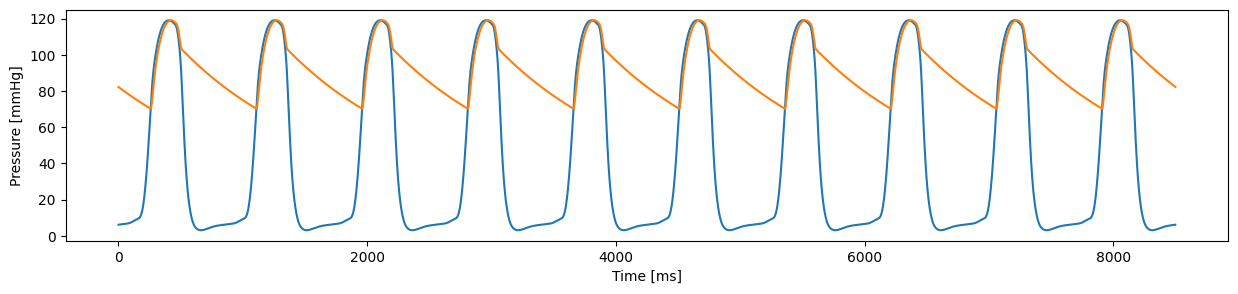
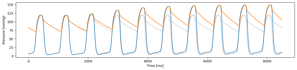
By default, it is turned on to control cardiac output and mean arterial pressure.
model1 = VanOsta2024()
model1.run(stable = True)
model1['Solver']['store_beats'] = 10
model1['PFC']['p0'] = 15000
model1.run(10)

# plot
fig = plt.figure(figsize=(15,3))
plt.plot(model['Solver']['t']*1e3, model['Cavity']['p'][:, ['cLv', 'SyArt']]/133, c=[0.8, 0.8, 0.8])
plt.plot(model1['Solver']['t']*1e3, model1['Cavity']['p'][:, ['cLv', 'SyArt']]/133)
plt.xlabel('Time [ms]')
plt.ylabel('Pressure [mmHg]')
fig
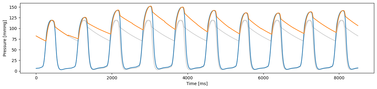
Pressure Flow Control off
You can turn pressure flow control off.
model2 = VanOsta2024()
model2.run(stable = True)
model2['Solver']['store_beats'] = 10
model2['PFC']['is_active'] = False
model2['Patch']['Sf_act'] *= 0.5
model2['Patch']['k1'] *= 1.2
model2.run(9)

# plot
fig = plt.figure(figsize=(15,3))
plt.plot(model['Solver']['t']*1e3, model['Cavity']['p'][:, ['cLv', 'SyArt']]/133, c=[0.8, 0.8, 0.8])
plt.plot(model2['Solver']['t']*1e3, model2['Cavity']['p'][:, ['cLv', 'SyArt']]/133)
plt.xlabel('Time [ms]')
plt.ylabel('Pressure [mmHg]')
fig
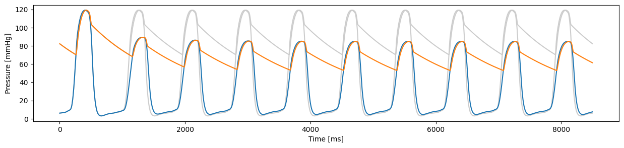
Volume control
The total blood volume can be a model input parameter.
model3 = VanOsta2024()
model3.run(stable = True)
model3['Solver']['store_beats'] = 10
model3['PFC']['is_volume_control'] = True
model3['PFC']['target_volume'] = 0.001

model3.run(9)

# plot
fig = plt.figure(figsize=(15,3))
plt.plot(model['Solver']['t']*1e3, model['Cavity']['p'][:, ['cLv', 'SyArt']]/133, c=[0.8, 0.8, 0.8])
plt.plot(model3['Solver']['t']*1e3, model3['Cavity']['p'][:, ['cLv', 'SyArt']]/133)
plt.xlabel('Time [ms]')
plt.ylabel('Pressure [mmHg]')
fig